Trajectory Analysis
PAGA
Partition-based graph abstraction (PAGA), is an algorithm which provides an interpretable graph-like map of the arising data manifold, based on estimating connectivity of manifold partitions [Wolf19].
Before running PAGA, we need to create a group of cluster results and a neigbobor pairwise matrix. Here we use mouse embryo data for demo. Download the example data first.
[1]:
import stereo as st
import warnings
warnings.filterwarnings('ignore')

# read data
data = st.io.read_h5ad('../data/Embyro/Embyro_E9.5.h5ad')

# preprocessing
data.tl.cal_qc()
data.tl.raw_checkpoint()
data.tl.normalize_total(target_sum=1e4)
data.tl.log1p()

# hvg
data.tl.highly_variable_genes(min_mean=0.0125, max_mean=3, min_disp=0.5, res_key='highly_variable_genes', n_top_genes=None)

data.tl.scale(zero_center=False)

# embedding
data.tl.pca(use_highly_genes=True, hvg_res_key='highly_variable_genes', n_pcs=20, res_key='pca', svd_solver='arpack')
data.tl.neighbors(pca_res_key='pca', n_pcs=30, res_key='neighbors', n_jobs=-1)
data.tl.umap(pca_res_key='pca', neighbors_res_key='neighbors', res_key='umap')
[2024-04-07 17:41:26][Stereo][42395][MainThread][140284015499072][st_pipeline][41][INFO]: start to run cal_qc...
[2024-04-07 17:41:26][Stereo][42395][MainThread][140284015499072][st_pipeline][44][INFO]: cal_qc end, consume time 0.2455s.
[2024-04-07 17:41:27][Stereo][42395][MainThread][140284015499072][st_pipeline][41][INFO]: start to run normalize_total...
[2024-04-07 17:41:27][Stereo][42395][MainThread][140284015499072][st_pipeline][44][INFO]: normalize_total end, consume time 0.2725s.
[2024-04-07 17:41:27][Stereo][42395][MainThread][140284015499072][st_pipeline][41][INFO]: start to run log1p...
[2024-04-07 17:41:27][Stereo][42395][MainThread][140284015499072][st_pipeline][44][INFO]: log1p end, consume time 0.1476s.
[2024-04-07 17:41:27][Stereo][42395][MainThread][140284015499072][st_pipeline][41][INFO]: start to run highly_variable_genes...
[2024-04-07 17:41:27][Stereo][42395][MainThread][140284015499072][st_pipeline][44][INFO]: highly_variable_genes end, consume time 0.3330s.
[2024-04-07 17:41:27][Stereo][42395][MainThread][140284015499072][st_pipeline][41][INFO]: start to run scale...
[2024-04-07 17:41:28][Stereo][42395][MainThread][140284015499072][st_pipeline][44][INFO]: scale end, consume time 0.4013s.
[2024-04-07 17:41:28][Stereo][42395][MainThread][140284015499072][st_pipeline][41][INFO]: start to run pca...
[2024-04-07 17:41:30][Stereo][42395][MainThread][140284015499072][st_pipeline][44][INFO]: pca end, consume time 1.7432s.
[2024-04-07 17:41:30][Stereo][42395][MainThread][140284015499072][st_pipeline][41][INFO]: start to run neighbors...
[2024-04-07 17:41:33][Stereo][42395][MainThread][140284015499072][st_pipeline][44][INFO]: neighbors end, consume time 3.7700s.
[2024-04-07 17:41:33][Stereo][42395][MainThread][140284015499072][st_pipeline][41][INFO]: start to run umap...
        completed  0  /  500 epochs
        completed  50  /  500 epochs
        completed  100  /  500 epochs
        completed  150  /  500 epochs
        completed  200  /  500 epochs
        completed  250  /  500 epochs
        completed  300  /  500 epochs
        completed  350  /  500 epochs
        completed  400  /  500 epochs
        completed  450  /  500 epochs
[2024-04-07 17:41:44][Stereo][42395][MainThread][140284015499072][st_pipeline][44][INFO]: umap end, consume time 10.6142s.
[2]:
data.tl.paga(groups='annotation', neighbors_key='neighbors')
[2024-04-07 17:41:44][Stereo][42395][MainThread][140284015499072][st_pipeline][77][INFO]: register algorithm paga to <stereo.core.st_pipeline.AnnBasedStPipeline object at 0x7f965c1e81f0>
We could obtain connectivities and connectivities_tree in the result of PAGA. connectivities_tree indicates cluster-to-cluster relation.
[3]:
data.tl.result['paga']
[3]:
{'connectivities': <12x12 sparse matrix of type '<class 'numpy.float64'>'
        with 90 stored elements in Compressed Sparse Row format>,
 'connectivities_tree': <12x12 sparse matrix of type '<class 'numpy.float64'>'
        with 11 stored elements in Compressed Sparse Row format>,
 'annotation_sizes': array([ 452, 1518,  200,  882,  283,  273,  382,   98,  337, 1008,  236,
         244]),
 'groups': 'annotation'}
Visualization for PAGA
[4]:
data.plt.paga_plot(
            adjacency='connectivities_tree', # keyword to use for paga or paga tree
            threshold=0.01, # prune edges lower than threshold
            layout='fr' # the method to layout each node
            )
[2024-04-07 17:41:44][Stereo][42395][MainThread][140284015499072][plot_collection][84][INFO]: register plot_func paga_plot to <stereo.plots.plot_collection.PlotCollection object at 0x7f960dbd6550>
[4]:

Note
The installation of the officially provided package fa2 which is necessary for layout='fa' is abnormal. In order to solve this problem, we recommend using our modified package for installation. the differences between the package we provide and the official package [ url ].
The first step is to download the installation package and unzip it.* The second step is to enter the directory where the decompressed file is located and use
python setup.py install.
[5]:
data.plt.draw_graph(
        adjacency='connectivities_tree',
        threshold=0.01,
        layout='fa'
        )
[2024-04-07 17:41:44][Stereo][42395][MainThread][140284015499072][plot_collection][84][INFO]: register plot_func draw_graph to <stereo.plots.plot_collection.PlotCollection object at 0x7f960dbd6550>
[5]:

[6]:
data.plt.paga_compare(
        adjacency='connectivities_tree',
        threshold=0.01
        )
[2024-04-07 17:49:37][Stereo][42395][MainThread][140284015499072][plot_collection][84][INFO]: register plot_func paga_compare to <stereo.plots.plot_collection.PlotCollection object at 0x7f960dbd6550>
[6]:

[7]:
data.plt.paga_compare(
        adjacency='connectivities',
        threshold=0.01
        )
[7]:

Cluster trajectory
Plot the cluster trajectory described by the result of PAGA.
[8]:
x_raw = data.position[:, 0]
y_raw = data.position[:, 1]

data.plt.plot_cluster_traj(
        data.tl.result['paga']['connectivities_tree'].todense(),
        x_raw,
        y_raw,
        data.cells['annotation'].to_numpy(),
        lower_thresh_not_equal=0.95,
        count_thresh=100,
        eps_co=30,
        check_surr_co=20,
        show_ticks=True,
        type_traj="straight",
        plotting_scale_width=50,
        )
[2024-04-07 17:49:38][Stereo][42395][MainThread][140284015499072][plot_collection][84][INFO]: register plot_func plot_cluster_traj to <stereo.plots.plot_collection.PlotCollection object at 0x7f960dbd6550>
[8]:
<Figure size 6400x4800 with 0 Axes>

DPT
The chronology of differentiated cells is essentially implicit in their single-cell expression products. Diffusion pseudotime (DPT) is an efficient way to estimate this order, which uses diffusion-like random walks to measure cell-to-cell metastasis [Haghverdi16]. DPT method enables the reconstruction of cellular development, identifying transient or metastable states, branching decisions, and differentiation endpoints.
As an example, we choose the 100th Spinal cord cell as the root cell.
[9]:
import numpy as np

# setting the `iroot` to data.tl.result
data.tl.result['iroot'] = np.flatnonzero(data.cells['annotation'] == 'Cavity')[100]  # 'Heart'
data.tl.dpt(n_branchings=0)
[2024-04-07 17:49:39][Stereo][42395][MainThread][140284015499072][st_pipeline][77][INFO]: register algorithm dpt to <stereo.core.st_pipeline.AnnBasedStPipeline object at 0x7f965c1e81f0>
[2024-04-07 17:49:39][Stereo][42395][MainThread][140284015499072][main][989][WARNING]: Trying to run `tl.dpt` without prior call of `tl.diffmap`. Falling back to `tl.diffmap` with default parameters.
[2024-04-07 17:49:39][Stereo][42395][MainThread][140284015499072][main][21][INFO]: computing Diffusion Maps using n_comps=15(=n_dcs)
[2024-04-07 17:49:39][Stereo][42395][MainThread][140284015499072][struct][732][INFO]: finished
[2024-04-07 17:49:40][Stereo][42395][MainThread][140284015499072][struct][793][INFO]:     eigenvalues of transition matrix
    [1.         0.9968214  0.9944742  0.99249655 0.991394   0.99011517
     0.98855114 0.9875123  0.9872849  0.9851326  0.98486674 0.983596
     0.98220223 0.980026   0.97919136]
[2024-04-07 17:49:40][Stereo][42395][MainThread][140284015499072][main][27][INFO]:     finished
added
    'X_diffmap', diffmap coordinates (stereo_exp_data.cellsm)
    'diffmap_evals', eigenvalues of transition matrix (stereo_exp_data.tl.result)
[2024-04-07 17:49:40][Stereo][42395][MainThread][140284015499072][main][1003][INFO]: computing Diffusion Pseudotime using n_dcs=10
[2024-04-07 17:49:40][Stereo][42395][MainThread][140284015499072][main][1028][INFO]:     finished
added
    'dpt_pseudotime', the pseudotime (stereo_exp_data.cells)
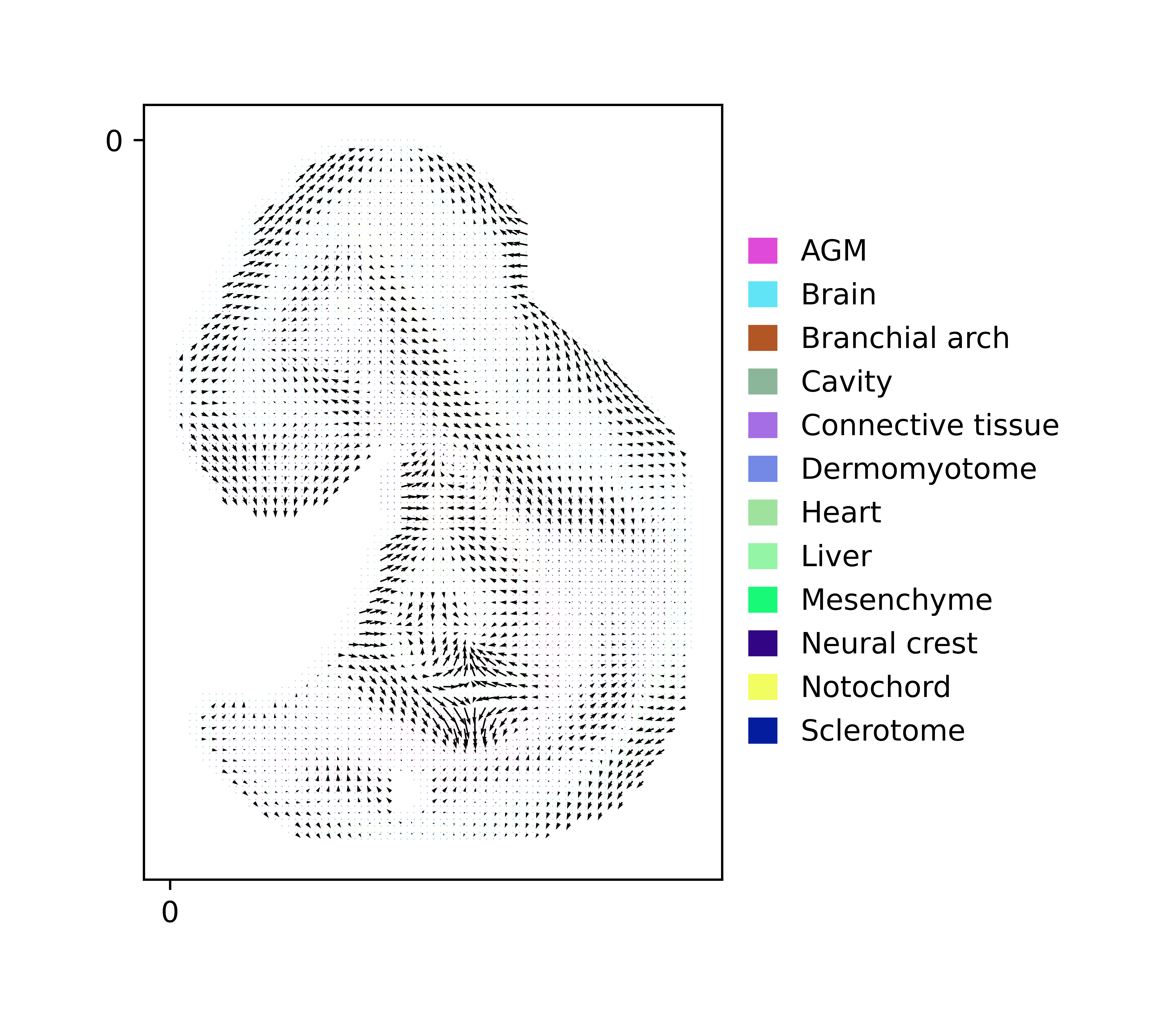
Vector plot
The stream-mode (set parameter type as stream) describes dpt as streams that flow from lower pseudotime to higher pseudotime. Background shows distribution of cell types or clusters, and it can take forms of either observations (set ‘background’ as ‘scatter’) or pixels (set ‘background’ as ‘field’).
We could also use the result to complete stream-mode plot.
[10]:
data.plt.plot_vec(
        data.position[:, 0] - data.position[:, 0].min(),
        data.position[:, 1] - data.position[:, 1].min(),
        data.cells['annotation'].to_numpy(),
        data.tl.result['dpt_pseudotime'],
        type='stream',
        line_width=0.5,
        background='field',
        num_pix=50,
        filter_type='gauss',
        sigma_val=1,
        radius_val=3,
        density=2,
        seed_val=0,
        num_legend_per_col=20,
        dpi_val=1000
        )
[2024-04-07 17:49:40][Stereo][42395][MainThread][140284015499072][plot_collection][84][INFO]: register plot_func plot_vec to <stereo.plots.plot_collection.PlotCollection object at 0x7f960dbd6550>
[10]:

[11]:
data.plt.plot_vec(
        data.position[:, 0] - data.position[:, 0].min(),
        data.position[:, 1] - data.position[:, 1].min(),
        data.cells['annotation'].to_numpy(),
        data.tl.result['dpt_pseudotime'],
        type='stream',
        line_width=0.5,
        background='scatter',
        num_pix=50,
        filter_type='gauss',
        sigma_val=1,
        radius_val=3,
        scatter_s=0.2,
        density=2,
        seed_val=0,
        num_legend_per_col=20,
        dpi_val=1000
        )
[11]:

We could also use the result to complete vector-mode plot.
[12]:
data.plt.plot_vec(
        data.position[:, 0] - data.position[:, 0].min(),
        data.position[:, 1] - data.position[:, 1].min(),
        data.cells['annotation'].to_numpy(),
        data.tl.result['dpt_pseudotime'],
        type='vec',
        background='field',
        num_pix=50,
        filter_type='gauss',
        sigma_val=2,
        radius_val=1,
        seed_val=0,
        dpi_val=1000
        )
[12]:

[13]:
data.plt.plot_vec(
        data.position[:, 0] - data.position[:, 0].min(),
        data.position[:, 1] - data.position[:, 1].min(),
        data.cells['annotation'].to_numpy(),
        data.tl.result['dpt_pseudotime'],
        type='vec',
        background='scatter',
        num_pix=50,
        filter_type='gauss',
        sigma_val=2,
        radius_val=1,
        scatter_s=0.2,
        seed_val=0,
        dpi_val=1000
        )
[13]:
[14]:
data.plt.plot_time_scatter(group='annotation', plotting_scale_width=50)
[2024-04-07 17:49:56][Stereo][42395][MainThread][140284015499072][plot_collection][84][INFO]: register plot_func plot_time_scatter to <stereo.plots.plot_collection.PlotCollection object at 0x7f960dbd6550>
[14]:

Distribution of marker genes over pseudotime
[15]:
data.tl.find_marker_genes(cluster_res_key='annotation', method='t_test', use_highly_genes=False, use_raw=True, res_key='marker_genes')
[2024-04-07 17:49:57][Stereo][42395][MainThread][140284015499072][st_pipeline][41][INFO]: start to run find_marker_genes...
[2024-04-07 17:50:00][Stereo][42395][MainThread][140284015499072][tool_base][122][INFO]: read group information, grouping by group column.
[2024-04-07 17:50:00][Stereo][42395][MainThread][140284015499072][tool_base][151][INFO]: start to run...
[2024-04-07 17:50:03][Stereo][42395][MainThread][140284015499072][tool_base][153][INFO]: end to run.
[2024-04-07 17:50:03][Stereo][42395][MainThread][140284015499072][st_pipeline][44][INFO]: find_marker_genes end, consume time 6.3101s.
[16]:
data.plt.plot_genes_in_pseudotime(
    marker_genes_res_key='marker_genes',
    group='Cavity',
    topn=5
)
[2024-04-07 17:50:03][Stereo][42395][MainThread][140284015499072][plot_collection][84][INFO]: register plot_func plot_genes_in_pseudotime to <stereo.plots.plot_collection.PlotCollection object at 0x7f960dbd6550>
[16]:

Temporal gene pattern for serially up & down regulated genes along trajectory
Stereopy also provideS a method to explore the genes that highly correlated to the development trajectory. The gene expression exhibits a certain pattern along the trajectory. For example, you can use time_series_analysis to find up or down-regulated genes during developmental trajectory.
[17]:
data.tl.time_series_analysis(
        run_method='tvg_marker',
        use_col='annotation',
        branch=['AGM', 'Brain', 'Branchial arch', 'Cavity'],
        p_val_combination='FDR'
        )
[2024-04-07 17:50:05][Stereo][42395][MainThread][140284015499072][st_pipeline][77][INFO]: register algorithm time_series_analysis to <stereo.core.st_pipeline.AnnBasedStPipeline object at 0x7f965c1e81f0>
[18]:
data.genes.to_df().sort_values('less_pvalue').iloc[:3]
[18]:
| n_cells_by_counts | mean_counts | log1p_mean_counts | pct_dropout_by_counts | total_counts | log1p_total_counts | n_cells | n_counts | mean_umi | means | dispersions | dispersions_norm | highly_variable | less_pvalue | greater_pvalue | logFC | |
|---|---|---|---|---|---|---|---|---|---|---|---|---|---|---|---|---|
| gene_short_name | ||||||||||||||||
| Nr2f2 | 184082 | 0.706283 | 0.534318 | 64.655012 | 367843 | 12.815414 | 4077 | 13934 | 3.417709 | 1.016122 | 0.844616 | -0.455328 | False | 0.001142 | 1.0 | -0.445506 |
| Rps14 | 512824 | 16.291674 | 2.850225 | 1.534326 | 8484948 | 15.953804 | 5861 | 242745 | 41.416994 | 3.494349 | 1.762277 | 0.859271 | False | 0.001611 | 1.0 | -0.052198 |
| Atp5j | 399663 | 3.313422 | 1.461732 | 23.262003 | 1725680 | 14.361132 | 5655 | 52523 | 9.287887 | 2.053444 | 1.205436 | -0.197009 | False | 0.007736 | 1.0 | -0.138287 |
[19]:
data.genes.to_df().sort_values('greater_pvalue').iloc[:3]
[19]:
| n_cells_by_counts | mean_counts | log1p_mean_counts | pct_dropout_by_counts | total_counts | log1p_total_counts | n_cells | n_counts | mean_umi | means | dispersions | dispersions_norm | highly_variable | less_pvalue | greater_pvalue | logFC | |
|---|---|---|---|---|---|---|---|---|---|---|---|---|---|---|---|---|
| gene_short_name | ||||||||||||||||
| Camk1d | 501169 | 20.675413 | 3.076179 | 3.772165 | 10768065 | 16.192095 | 4210 | 19946 | 4.737767 | 1.360882 | 2.281406 | 2.063298 | True | 1.000000 | 0.021118 | 0.285520 |
| Gm47253 | 139 | 0.000353 | 0.000353 | 99.973311 | 184 | 5.220356 | 9 | 12 | 1.333333 | 0.003194 | 1.982448 | 2.567851 | False | 0.996286 | 0.530018 | 9.019124 |
| Gm49165 | 772 | 0.001561 | 0.001560 | 99.851771 | 813 | 6.701960 | 23 | 30 | 1.304348 | 0.005304 | 0.715936 | 0.273936 | False | 0.991585 | 0.543550 | 9.010276 |
[20]:
data.plt.boxplot_transit_gene(
                use_col='annotation',
                branch=['AGM', 'Brain', 'Branchial arch', 'Cavity'],
                genes=list(data.genes.to_df().sort_values('greater_pvalue').iloc[:3].index) + list(data.genes.to_df().sort_values('less_pvalue').iloc[:3].index)
                )
[2024-04-07 17:50:13][Stereo][42395][MainThread][140284015499072][plot_collection][84][INFO]: register plot_func boxplot_transit_gene to <stereo.plots.plot_collection.PlotCollection object at 0x7f960dbd6550>
[20]:

Fuzzy’C means to cluster genes on spatial & temporal pattern
Except for up or down regulated genes, there is the other expression pattern also important. Stereopy considers both temporal and spatial information and based on which cluster genes into serveral groups.
[21]:
data.tl.time_series_analysis(run_method='other', cluster_number=4)
[22]:
data.plt.fuzz_cluster_plot(
        use_col='annotation',
        branch=['AGM', 'Brain', 'Branchial arch', 'Cavity'],
        threshold = 'p99.9',
        n_col = 4,
        summary_trend=True,
        width = None,
        height = None
        )
[2024-04-07 17:50:19][Stereo][42395][MainThread][140284015499072][plot_collection][84][INFO]: register plot_func fuzz_cluster_plot to <stereo.plots.plot_collection.PlotCollection object at 0x7f960dbd6550>
[22]:

[ ]: