3D Gene Regulatory Network
Gene regulatory networks (GRNs) are intricate systems that govern the complex interactions between genes and their regulatory elements, playing a fundamental role in controlling gene expression patterns within cells. These networks consist of genes, transcription factors, and other regulatory molecules that work in concert to determine when and to what extent genes are activated or repressed [VandeSande20].
Here, in Stereopy, we provide a computational tool specifically designed for inferring TF-centered, spatial GRNs using spatially resolved transcriptomics (SRT) data. To ensure accurate GRN inference, we employ pre-defined transcription factors (TFs) and utilize cis-regulatory element activity inference (CIS) as part of the methodology. This approach allows us to capture the regulatory interactions and dynamics of gene expression at a spatial level, providing valuable insights into the organization and control of gene regulatory networks in complex biological systems [Fang23].
It is important to note that the GRN analysis discussed here forms a crucial segment of the comprehensive NicheReg3D pipeline.
This part shows how to perform the function of Gene Regulatory Network on 3D data (several samples).
MSData construction
We use Drosophila melanogaster data to simulate a 3D model. Download the example data first.
[1]:
import os
from natsort import natsorted
import stereo as st
from stereo.core.ms_data import MSData
from stereo.core.ms_pipeline import slice_generator
import warnings
warnings.filterwarnings('ignore')
# prepara for input directory
# data_dir = './Demo_3D/3D_AnnData_0.8.0'
data_dir = '../data/mouse_embryo_heart_slices/'
files = []
for i in os.listdir(data_dir):
files.append(os.path.join(data_dir, i))
# ensure data order by naming them regularly
files = natsorted(files)
# construct MSData object
ms_data = MSData(_relationship='continuous', _var_type='intersect')
# add all samples into MSData
for sample in files:
ms_data += st.io.read_h5ad(sample, bin_type='bins', bin_size=1)


Coordinate calibration
In the analysis related to 3D data, we will recontruct 3D mesh in visualizing stage. It means that three-dimensional coordinates are needed, and we have to run ms_dta.tl.paste for better visualization. This function recalculates x-coordinate and y-coordinate, acoording to expression matrix, for that matter you could decide where to perform it, before filtering and normalization or after them.
[2]:
# ms_data.tl.paste()
After loading files into MSData, you need to perform integration. The parameter space_between represents the distance between each adjacent pair, which will be used for z-coordinate of each sample. If data already has z-coordinate information, it will be used firstly, or you have to set space_between acoording to biochemical experiment records.
Note
ms_data.integrate() is necessarily to be performed after data loading. Default method is intersect, which means to take the intersection of genes (var) for subsequent multi-sample analysis. After integration, _var_type shows the intersect gene number from 0 to 13668. Otherwise here also provide union method.
[3]:
ms_data.integrate(space_between='1um')
ms_data
[3]:
ms_data: {'0': (870, 30254), '1': (344, 30254), '2': (195, 30254), '3': (190, 30254), '4': (34, 30254), '5': (493, 30254), '6': (285, 30254), '7': (753, 30254), '8': (731, 30254), '9': (412, 30254), '10': (541, 30254), '11': (1103, 30254), '12': (1051, 30254), '13': (1293, 30254), '14': (1269, 30254), '15': (1503, 30254), '16': (1872, 30254), '17': (2071, 30254), '18': (2124, 30254), '19': (2221, 30254), '20': (2198, 30254), '21': (1992, 30254), '22': (1837, 30254), '23': (2010, 30254), '24': (1977, 30254), '25': (2078, 30254), '26': (2255, 30254), '27': (664, 30254), '28': (2343, 30254), '29': (2168, 30254), '30': (895, 30254), '31': (1478, 30254), '32': (1691, 30254), '33': (1370, 30254), '34': (2911, 30254), '35': (2501, 30254), '36': (2194, 30254), '37': (2023, 30254), '38': (1443, 30254), '39': (1190, 30254), '40': (1461, 30254), '41': (2760, 30254), '42': (2662, 30254), '43': (2391, 30254), '44': (2490, 30254), '45': (2104, 30254), '46': (1557, 30254), '47': (2253, 30254), '48': (1969, 30254), '49': (2448, 30254), '50': (2487, 30254), '51': (2226, 30254), '52': (2124, 30254), '53': (1282, 30254), '54': (1098, 30254), '55': (873, 30254), '56': (661, 30254), '57': (454, 30254), '58': (423, 30254)}
num_slice: 59
names: ['0', '1', '2', '3', '4', '5', '6', '7', '8', '9', '10', '11', '12', '13', '14', '15', '16', '17', '18', '19', '20', '21', '22', '23', '24', '25', '26', '27', '28', '29', '30', '31', '32', '33', '34', '35', '36', '37', '38', '39', '40', '41', '42', '43', '44', '45', '46', '47', '48', '49', '50', '51', '52', '53', '54', '55', '56', '57', '58']
obs: ['batch']
var: []
relationship: continuous
var_type: intersect to 30254
mss: []
Preprocessing
scope and mode are crucial parameters in basic multi-sample analysis and correlated funcitons.
scope, similar to list, means which samples used for analysis.mode, like a switch, shows that analysis is performed on single sample or multi samples,integrateandisolated. It is easy to distinguish processing modes.
[4]:
ms_data.tl.cal_qc(scope=slice_generator[:],mode='integrate')
ms_data.tl.raw_checkpoint()
[2023-11-15 13:58:11][Stereo][39122][MainThread][140302246872896][ms_pipeline][131][INFO]: data_obj(idx=0) in ms_data start to run cal_qc
[2023-11-15 13:58:11][Stereo][39122][MainThread][140302246872896][st_pipeline][41][INFO]: start to run cal_qc...
[2023-11-15 13:58:11][Stereo][39122][MainThread][140302246872896][st_pipeline][44][INFO]: cal_qc end, consume time 0.4671s.
[2023-11-15 13:58:11][Stereo][39122][MainThread][140302246872896][ms_pipeline][131][INFO]: data_obj(idx=0) in ms_data start to run raw_checkpoint
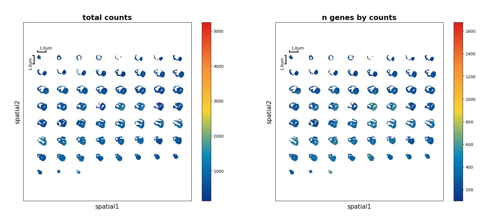
Show the spatial scatter figure of QC distribution. In Multi-sample analysis, serveral parameters are added here for better visual presentation.
[5]:
ms_data.plt.spatial_scatter(
scope=slice_generator[:],
mode='integrate',
plotting_scale_width=2, # the width of scale
reorganize_coordinate=8, # the number of plots in each row
# horizontal_offset_additional=20, # adjustment for horizontal distance
# vertical_offset_additional=20 # adjustment for vertical distance
)
[2023-11-15 13:58:12][Stereo][39122][MainThread][140302246872896][ms_pipeline][131][INFO]: data_obj(idx=0) in ms_data start to run spatial_scatter
[5]:
Preparation of Input
Before performing the function, make sure the preparation of following input files:
Spatially resolved transcriptomics data: the matrix of gene expression for each single cell. Each column represents a gene, and each row represents a SRT sample. Values in the matrix are typically gene expression levels, either raw counts or normalized expression (raw counts prefered). SRT expression matrix of bin200 in the mouse brain generated by Stereo-seq is used here, through example data.
Transcription factor gene list: a list of transcription factors of interest. This list is requried for the network inference step. Data can be downloaded through pySCENIC_TF_list and TF_lists.
Ranked whole genome databases: Databases ranking the whole genome of species of interest based on transcription factors in feather v2 format. Data can typically be downloaded from public databases, through cisTarget databases.
Motif to TF annotation databases: Motif databases (in tbl format) serve as a reference for identifying potential TF binding sites in the genome and inferring the regulatory relationships between TFs and target genes. Data can be downloaded through Motif2TF annotations.
Note
Please note that in the 3D gene regulatory network, the z coordinate information added in the calculation can only be used to calculate the TF-gene-importance results using the hotspot method [DeTomaso21].
[6]:
tfs_fn = '../data/grn/test_mm_mgi_tfs.txt'
database_fn = '../data/grn/mm10_10kbp_up_10kbp_down_full_tx_v10_clust.genes_vs_motifs.rankings.feather'
motif_anno_fn = '../data/grn/motifs-v10nr_clust-nr.mgi-m0.001-o0.0.tbl'
# ms_data.tl.regulatory_network_inference(database_fn, motif_anno_fn, tfs_fn, save=True, num_workers=10, method='hotspot', ThreeD_slice=True, auc_threshold=0.05, prune_kwargs={'rank_threshold': 8000, 'auc_threshold': 0.05}, mode='integrate')
ms_data.tl.regulatory_network_inference(
database_fn,
motif_anno_fn,
tfs_fn,
save_regulons=True,
num_workers=20,
method='hotspot',
ThreeD_slice=True,
use_raw=True,
mode='integrate'
)
[2023-11-15 13:58:14][Stereo][39122][MainThread][140302246872896][ms_pipeline][121][INFO]: register algorithm regulatory_network_inference to <class 'stereo.core.stereo_exp_data.StereoExpData'>-140302023674512
[2023-11-15 13:58:14][Stereo][39122][MainThread][140302246872896][main][96][INFO]: the raw expression matrix will be used.
[2023-11-15 13:59:19][Stereo][39122][MainThread][140302246872896][main][386][INFO]: Loading ranked database...
[2023-11-15 13:59:19][Stereo][39122][MainThread][140302246872896][main][125][INFO]: If data belongs to 3D, it only can be runned as hotspot method now
[2023-11-15 13:59:19][Stereo][39122][MainThread][140302246872896][main][229][INFO]: cached file not found, running hotspot now
[2023-11-15 14:04:08][Stereo][39122][MainThread][140302246872896][main][254][INFO]: compute_autocorrelations()
100%|██████████| 14405/14405 [01:33<00:00, 154.04it/s]
[2023-11-15 14:05:57][Stereo][39122][MainThread][140302246872896][main][256][INFO]: compute_autocorrelations() done
[2023-11-15 14:05:57][Stereo][39122][MainThread][140302246872896][main][259][INFO]: compute_local_correlations
Computing pair-wise local correlation on 2513 features...
100%|██████████| 2513/2513 [00:27<00:00, 90.55it/s]
100%|██████████| 3156328/3156328 [25:20<00:00, 2075.74it/s]
[2023-11-15 14:33:07][Stereo][39122][MainThread][140302246872896][main][262][INFO]: Network Inference DONE
[2023-11-15 14:33:07][Stereo][39122][MainThread][140302246872896][main][263][INFO]: Hotspot: create 2513 features
[2023-11-15 14:33:07][Stereo][39122][MainThread][140302246872896][main][264][INFO]: (2513, 2513)
[2023-11-15 14:33:07][Stereo][39122][MainThread][140302246872896][main][269][INFO]: detected 63 predefined TF in data
2023-11-15 14:33:36,688 - pyscenic.utils - INFO - Calculating Pearson correlations.
INFO:pyscenic.utils:Calculating Pearson correlations.
2023-11-15 14:33:37,447 - pyscenic.utils - WARNING - Note on correlation calculation: the default behaviour for calculating the correlations has changed after pySCENIC verion 0.9.16. Previously, the default was to calculate the correlation between a TF and target gene using only cells with non-zero expression values (mask_dropouts=True). The current default is now to use all cells to match the behavior of the R verision of SCENIC. The original settings can be retained by setting 'rho_mask_dropouts=True' in the modules_from_adjacencies function, or '--mask_dropouts' from the CLI.
Dropout masking is currently set to [False].
WARNING:pyscenic.utils:Note on correlation calculation: the default behaviour for calculating the correlations has changed after pySCENIC verion 0.9.16. Previously, the default was to calculate the correlation between a TF and target gene using only cells with non-zero expression values (mask_dropouts=True). The current default is now to use all cells to match the behavior of the R verision of SCENIC. The original settings can be retained by setting 'rho_mask_dropouts=True' in the modules_from_adjacencies function, or '--mask_dropouts' from the CLI.
Dropout masking is currently set to [False].
2023-11-15 14:34:08,578 - pyscenic.utils - INFO - Creating modules.
INFO:pyscenic.utils:Creating modules.
[2023-11-15 14:34:22][Stereo][39122][MainThread][140302246872896][main][439][INFO]: cached file not found, running prune modules now
[########################################] | 100% Completed | 423.25 s
[2023-11-15 14:41:27][Stereo][39122][MainThread][140302246872896][main][483][INFO]: cached file not found, calculating auc_activity_level now
Create regulons from a dataframe of enriched features.
Additional columns saved: []
Note
If AssertionError: assert maxauc > 0 is thrown, it may be due to most of the genes are not mapped to the genome ranking databases or the majority of regulons’ target genes have low weights, you can try to set auc_threshold to lower and/or rank_threshold to higher to avoid this error.
For example:
ms_data.tl.regulatory_network_inference(database_fn, motif_anno_fn, tfs_fn, save=True, num_workers=10, method=’hotspot’, ThreeD_slice=True, auc_threshold=0.1, prune_kwargs={‘rank_threshold’: 4000, ‘auc_threshold’: 0.1}, mode=’integrate’)
Observation of results
[7]:
ms_data
[7]:
ms_data: {'0': (870, 30254), '1': (344, 30254), '2': (195, 30254), '3': (190, 30254), '4': (34, 30254), '5': (493, 30254), '6': (285, 30254), '7': (753, 30254), '8': (731, 30254), '9': (412, 30254), '10': (541, 30254), '11': (1103, 30254), '12': (1051, 30254), '13': (1293, 30254), '14': (1269, 30254), '15': (1503, 30254), '16': (1872, 30254), '17': (2071, 30254), '18': (2124, 30254), '19': (2221, 30254), '20': (2198, 30254), '21': (1992, 30254), '22': (1837, 30254), '23': (2010, 30254), '24': (1977, 30254), '25': (2078, 30254), '26': (2255, 30254), '27': (664, 30254), '28': (2343, 30254), '29': (2168, 30254), '30': (895, 30254), '31': (1478, 30254), '32': (1691, 30254), '33': (1370, 30254), '34': (2911, 30254), '35': (2501, 30254), '36': (2194, 30254), '37': (2023, 30254), '38': (1443, 30254), '39': (1190, 30254), '40': (1461, 30254), '41': (2760, 30254), '42': (2662, 30254), '43': (2391, 30254), '44': (2490, 30254), '45': (2104, 30254), '46': (1557, 30254), '47': (2253, 30254), '48': (1969, 30254), '49': (2448, 30254), '50': (2487, 30254), '51': (2226, 30254), '52': (2124, 30254), '53': (1282, 30254), '54': (1098, 30254), '55': (873, 30254), '56': (661, 30254), '57': (454, 30254), '58': (423, 30254)}
num_slice: 59
names: ['0', '1', '2', '3', '4', '5', '6', '7', '8', '9', '10', '11', '12', '13', '14', '15', '16', '17', '18', '19', '20', '21', '22', '23', '24', '25', '26', '27', '28', '29', '30', '31', '32', '33', '34', '35', '36', '37', '38', '39', '40', '41', '42', '43', '44', '45', '46', '47', '48', '49', '50', '51', '52', '53', '54', '55', '56', '57', '58']
obs: ['batch', 'total_counts', 'n_genes_by_counts', 'pct_counts_mt']
var: ['n_cells', 'n_counts', 'mean_umi']
relationship: continuous
var_type: intersect to 30254
mss: ["scope_[0,1,2,3,4,5,6,7,8,9,10,11,12,13,14,15,16,17,18,19,20,21,22,23,24,25,26,27,28,29,30,31,32,33,34,35,36,37,38,39,40,41,42,43,44,45,46,47,48,49,50,51,52,53,54,55,56,57,58]:['regulatory_network_inference']"]
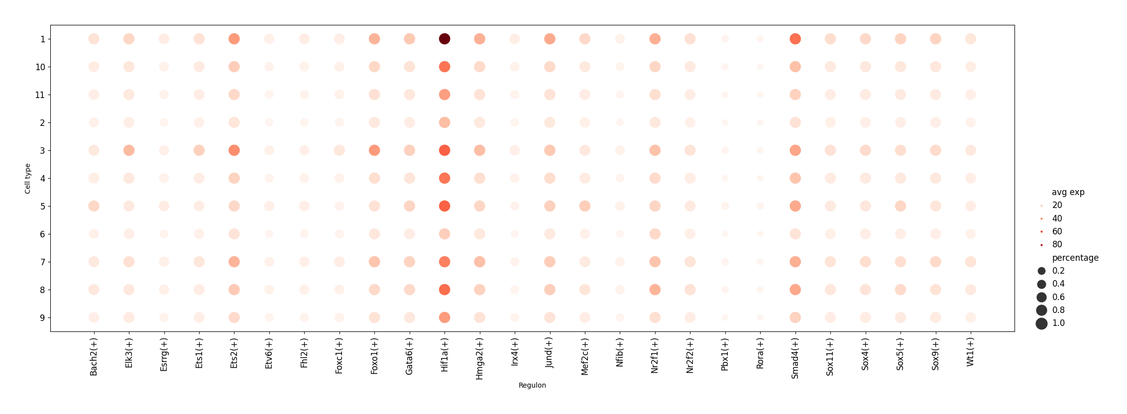
AUCell enrichment scores quantify activity of each regulon (a gene set) in each cell. In other words, the AUC represents the proportion of expressed genes in the signature and their relative expression values compared to the other genes within the cell.
[ ]:
scope_key = 'scope_[0,1,2,3,4,5,6,7,8,9,10,11,12,13,14,15,16,17,18,19,20,21,22,23,24,25,26,27,28,29,30,31,32,33,34,35,36,37,38,39,40,41,42,43,44,45,46,47,48,49,50,51,52,53,54,55,56,57,58]'
[ ]:
ms_data.mss[scope_key]['regulatory_network_inference']['auc_matrix']
Index of relative importance between TFs and their target genes.
[ ]:
ms_data.mss[scope_key]['regulatory_network_inference']['adjacencies']
Note
Please note that for multi samples, batch correction can be performed before clustering if necessary.
Clustering
[10]:
# normalization
ms_data.tl.normalize_total(scope=slice_generator[:],mode='integrate', target_sum=10000)
ms_data.tl.log1p(scope=slice_generator[:],mode='integrate')
ms_data.tl.scale(scope=slice_generator[:],mode='integrate', max_value=10, zero_center=True)
# embedding
ms_data.tl.pca(scope=slice_generator[:],mode='integrate', use_highly_genes=False, n_pcs=30, res_key='pca')
# batch correction
ms_data.tl.batches_integrate(scope=slice_generator[:],mode='integrate', pca_res_key='pca', res_key='pca_integrated')
# clustering
ms_data.tl.neighbors(scope=slice_generator[:],mode='integrate', pca_res_key='pca_integrated', n_pcs=30, res_key='neighbors_integrated')
ms_data.tl.leiden(scope=slice_generator[:],mode='integrate', neighbors_res_key='neighbors_integrated', res_key='leiden')
[2023-11-15 15:02:23][Stereo][39122][MainThread][140302246872896][ms_pipeline][131][INFO]: data_obj(idx=0) in ms_data start to run normalize_total
[2023-11-15 15:02:23][Stereo][39122][MainThread][140302246872896][st_pipeline][41][INFO]: start to run normalize_total...
[2023-11-15 15:02:23][Stereo][39122][MainThread][140302246872896][st_pipeline][44][INFO]: normalize_total end, consume time 0.3283s.
[2023-11-15 15:02:23][Stereo][39122][MainThread][140302246872896][ms_pipeline][131][INFO]: data_obj(idx=0) in ms_data start to run log1p
[2023-11-15 15:02:23][Stereo][39122][MainThread][140302246872896][st_pipeline][41][INFO]: start to run log1p...
[2023-11-15 15:02:25][Stereo][39122][MainThread][140302246872896][st_pipeline][44][INFO]: log1p end, consume time 1.6346s.
[2023-11-15 15:02:25][Stereo][39122][MainThread][140302246872896][ms_pipeline][131][INFO]: data_obj(idx=0) in ms_data start to run scale
[2023-11-15 15:02:25][Stereo][39122][MainThread][140302246872896][st_pipeline][41][INFO]: start to run scale...
[2023-11-15 15:03:23][Stereo][39122][MainThread][140302246872896][scale][53][INFO]: Truncate at max_value 10
[2023-11-15 15:03:31][Stereo][39122][MainThread][140302246872896][st_pipeline][44][INFO]: scale end, consume time 65.7160s.
[2023-11-15 15:03:31][Stereo][39122][MainThread][140302246872896][ms_pipeline][131][INFO]: data_obj(idx=0) in ms_data start to run pca
[2023-11-15 15:03:31][Stereo][39122][MainThread][140302246872896][st_pipeline][41][INFO]: start to run pca...
[2023-11-15 15:05:30][Stereo][39122][MainThread][140302246872896][st_pipeline][44][INFO]: pca end, consume time 119.4342s.
[2023-11-15 15:05:30][Stereo][39122][MainThread][140302246872896][ms_pipeline][131][INFO]: data_obj(idx=0) in ms_data start to run batches_integrate
[2023-11-15 15:05:30][Stereo][39122][MainThread][140302246872896][st_pipeline][41][INFO]: start to run batches_integrate...
2023-11-15 15:06:03,415 - harmonypy - INFO - Iteration 1 of 10
INFO:harmonypy:Iteration 1 of 10
2023-11-15 15:25:25,651 - harmonypy - INFO - Iteration 2 of 10
INFO:harmonypy:Iteration 2 of 10
2023-11-15 15:44:00,561 - harmonypy - INFO - Iteration 3 of 10
INFO:harmonypy:Iteration 3 of 10
2023-11-15 16:02:32,327 - harmonypy - INFO - Converged after 3 iterations
INFO:harmonypy:Converged after 3 iterations
[2023-11-15 16:02:32][Stereo][39122][MainThread][140302246872896][st_pipeline][44][INFO]: batches_integrate end, consume time 3421.7228s.
[2023-11-15 16:02:32][Stereo][39122][MainThread][140302246872896][ms_pipeline][131][INFO]: data_obj(idx=0) in ms_data start to run neighbors
[2023-11-15 16:02:32][Stereo][39122][MainThread][140302246872896][st_pipeline][41][INFO]: start to run neighbors...
[2023-11-15 16:03:14][Stereo][39122][MainThread][140302246872896][st_pipeline][44][INFO]: neighbors end, consume time 41.9798s.
[2023-11-15 16:03:14][Stereo][39122][MainThread][140302246872896][ms_pipeline][131][INFO]: data_obj(idx=0) in ms_data start to run leiden
[2023-11-15 16:03:14][Stereo][39122][MainThread][140302246872896][st_pipeline][41][INFO]: start to run leiden...
[2023-11-15 16:04:26][Stereo][39122][MainThread][140302246872896][st_pipeline][44][INFO]: leiden end, consume time 71.9816s.
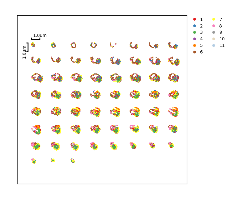
Display the visualization of clustering.
[11]:
ms_data.plt.cluster_scatter(
scope=slice_generator[:],
mode='integrate',
res_key='leiden',
dot_size=4,
plotting_scale_width=2,
reorganize_coordinate=8,
# horizontal_offset_additional=20,
# vertical_offset_additional=30
)
[2023-11-15 16:04:26][Stereo][39122][MainThread][140302246872896][ms_pipeline][131][INFO]: data_obj(idx=0) in ms_data start to run cluster_scatter
[11]:
Visualization of network
[12]:
ms_data.plt.grn_dotplot(
scope=slice_generator[:],
mode='integrate',
cluster_res_key='leiden',
network_res_key='regulatory_network_inference'
)
[2023-11-15 16:04:30][Stereo][39122][MainThread][140302246872896][ms_pipeline][128][INFO]: register plot_func grn_dotplot to <class 'stereo.core.stereo_exp_data.StereoExpData'>-140302023674512
INFO:matplotlib.category:Using categorical units to plot a list of strings that are all parsable as floats or dates. If these strings should be plotted as numbers, cast to the appropriate data type before plotting.
INFO:matplotlib.category:Using categorical units to plot a list of strings that are all parsable as floats or dates. If these strings should be plotted as numbers, cast to the appropriate data type before plotting.
[12]:
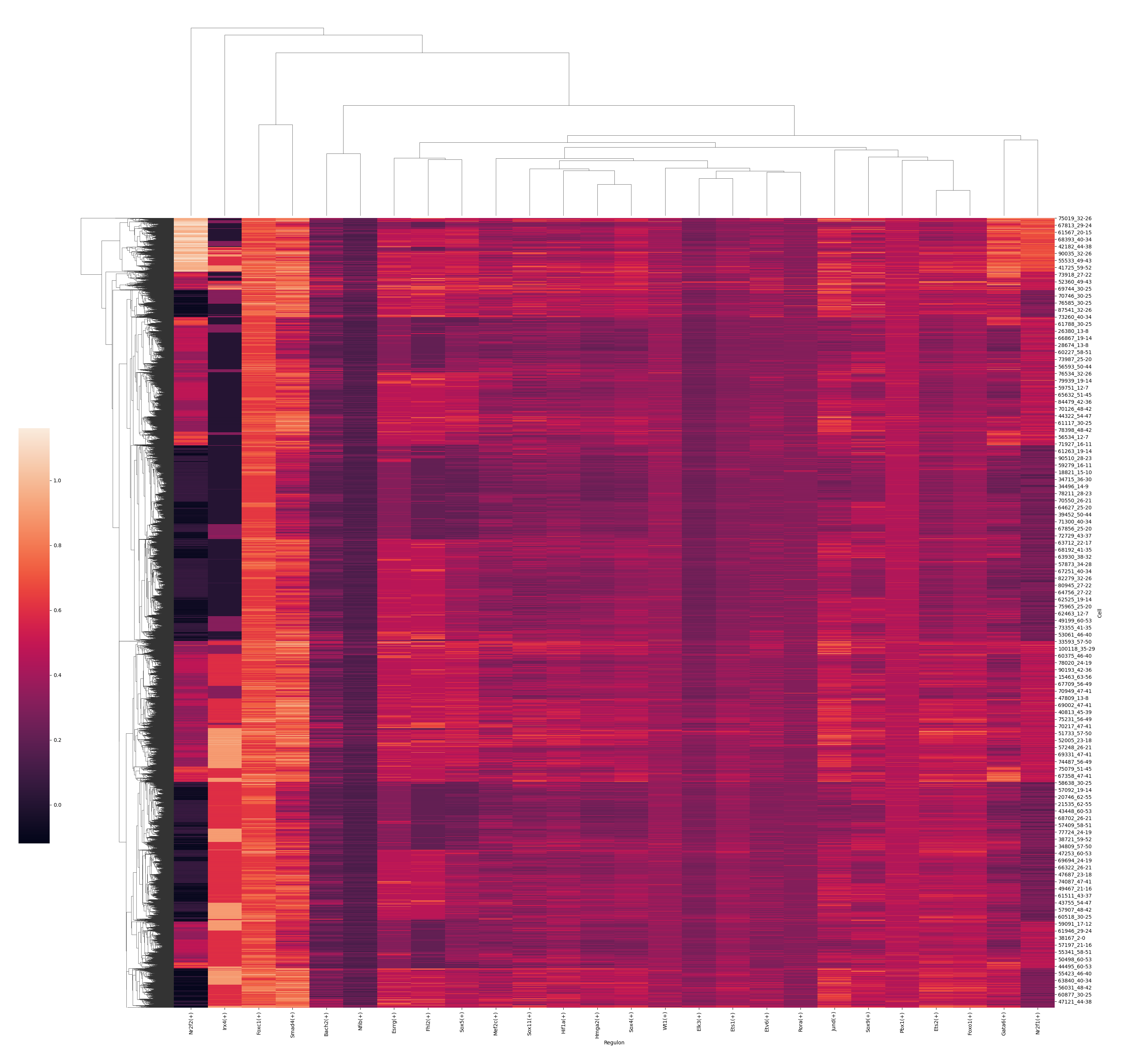
[13]:
ms_data.plt.auc_heatmap(
scope=slice_generator[:],
mode='integrate',
network_res_key='regulatory_network_inference',
width=28,
height=28
)
[2023-11-15 16:05:19][Stereo][39122][MainThread][140302246872896][ms_pipeline][128][INFO]: register plot_func auc_heatmap to <class 'stereo.core.stereo_exp_data.StereoExpData'>-140302023674512
[2023-11-15 16:05:19][Stereo][39122][MainThread][140302246872896][plot_grn][263][INFO]: Generating auc heatmap plot
[13]:
<seaborn.matrix.ClusterGrid at 0x7f95f83cf5b0>
[14]:
ms_data.plt.auc_heatmap_by_group(
scope=slice_generator[:],
mode='integrate',
network_res_key='regulatory_network_inference',
cluster_res_key='leiden',
top_n_feature=5
)
[2023-11-15 16:24:58][Stereo][39122][MainThread][140302246872896][ms_pipeline][128][INFO]: register plot_func auc_heatmap_by_group to <class 'stereo.core.stereo_exp_data.StereoExpData'>-140302023674512
[14]:
<seaborn.matrix.ClusterGrid at 0x7f93d84a0790>

[16]:
ms_data.plt.spatial_scatter_by_regulon(
scope=slice_generator[:],
mode='integrate',
reg_name='Foxc1(+)',
network_res_key='regulatory_network_inference',
plotting_scale_width=2, reorganize_coordinate=8,
# horizontal_offset_additional=20, vertical_offset_additional=30
)
[2023-11-15 16:48:26][Stereo][39122][MainThread][140302246872896][ms_pipeline][128][INFO]: register plot_func spatial_scatter_by_regulon to <class 'stereo.core.stereo_exp_data.StereoExpData'>-140302023674512
[2023-11-15 16:48:27][Stereo][39122][MainThread][140302246872896][plot_grn][331][INFO]: Please adjust the dot_size to prevent dots from covering each other
[16]:

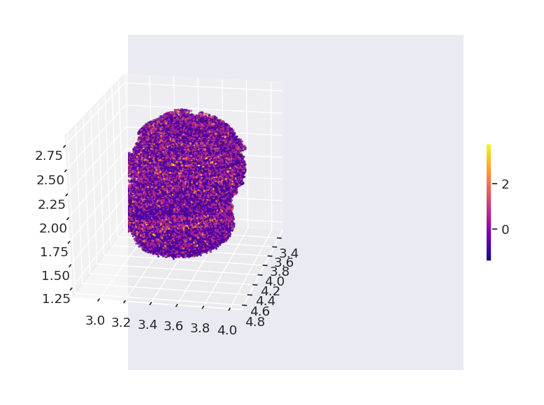
3D spatial expression map of the regulon can also be visualized using the function spatial_scatter_by_regulon_3D. The observation angle can be adjusted using the view_horizontal and view_vertical parameters.
[17]:
ms_data.plt.spatial_scatter_by_regulon_3D(
scope=slice_generator[:],
mode='integrate',
reg_name='Foxc1(+)',
view_horizontal=10,
view_vertical=20,
show_axis=True,
network_res_key='regulatory_network_inference'
)
[2023-11-15 16:48:47][Stereo][39122][MainThread][140302246872896][ms_pipeline][128][INFO]: register plot_func spatial_scatter_by_regulon_3D to <class 'stereo.core.stereo_exp_data.StereoExpData'>-140302023674512
Note
Please note that for multi samples, batch correction can be performed before clusteringif necessary.
[18]:
ms_data.plt.start_vt3d_browser(
scope=slice_generator[:],
mode='integrate',
grn_res_key='regulatory_network_inference',
cluster_res_key='leiden'
)
[2023-11-15 18:20:13][Stereo][39122][MainThread][140302246872896][ms_pipeline][128][INFO]: register plot_func start_vt3d_browser to <class 'stereo.core.stereo_exp_data.StereoExpData'>-140302023674512
Display 3D mesh in notebook.
Note
If you don’t run the notebook locally, you need to specify the IP of host on which this notebook is ran by parameter ip.
[ ]:
# ms_data.plt.display_3d_grn(scope=slice_generator[:],mode='integrate', ip='172.16.18.15')
ms_data.plt.display_3d_grn(scope=slice_generator[:],mode='integrate')
