Quick Start (Square Bin)
In this case, we use spatial expression matrix of bin1(bin_size is defined beblow) in the mouse brain generated by Stereo-seq for downstream analysis.
Note
Download the notebook of Quick Start. You can download all notebooks of Stereopy-tutorial on Github.
Introduction of raw data
GEM and GEF
There are two types of Stereo-seq data, GEM and GEF. The format of original expression matrix of GEM file is as follows: x, y are the spatial position of the gene in tissue section, and MIDCount is the number of gene expression. ExonCount is the number of exons expression only in GEM file, which is generated by spatial_RNA_visualization_v5 in SAP or SAW (version >= 5.1.3).

More information of GEF file is in the format documentation. Usually, we recommend using GEF format of which reading speed is much faster than GEM.
Bin size
The resolution of Stereo-seq technology is up to nanometer level, where nanopore radius of bin1 is 250 nm.
Generally, bin_size parameter is set to combine the nanopores within a certain range into a bin unit. For instance, the side length of the bin unit is approximately 10 or 14 microns when bin_size is set to 20, according to different center-to-center distances, like 500 nm or 715 nm.


After the combination according to a certain bin_size, we will uniformly generate data into the format of StereoExpData.
Performance
At the end of this part, we display the running performance of different bin_sizes to those who are handling mass data and more concerned about computational performance. Welcome to come back here after having finished this example. Also, similar performing tests come up elsewhere in Stereopy.
Reading data
Firstly, download our example data and import Stereopy.
[1]:
import stereo as st
import warnings
warnings.filterwarnings('ignore')
Get the version information of Stereopy.
[2]:
st.__version__
[2]:
'1.1.0'
Get attributes of the GEF file.
[3]:
data_path = '../data/SS200000135TL_D1.tissue.gef'
st.io.read_gef_info(data_path)
[2024-01-17 10:19:46][Stereo][3643][MainThread][140100178437952][reader][1317][INFO]: This is GEF file which contains traditional bin infomation.
[2024-01-17 10:19:46][Stereo][3643][MainThread][140100178437952][reader][1318][INFO]: bin_type: bins
[2024-01-17 10:19:46][Stereo][3643][MainThread][140100178437952][reader][1321][INFO]: Bin size list: ['bin1']
[2024-01-17 10:19:46][Stereo][3643][MainThread][140100178437952][reader][1327][INFO]: Resolution: 500
[2024-01-17 10:19:46][Stereo][3643][MainThread][140100178437952][reader][1330][INFO]: Gene count: 24302
[2024-01-17 10:19:46][Stereo][3643][MainThread][140100178437952][reader][1339][INFO]: offsetX: 0
[2024-01-17 10:19:46][Stereo][3643][MainThread][140100178437952][reader][1342][INFO]: offsetY: 0
[2024-01-17 10:19:46][Stereo][3643][MainThread][140100178437952][reader][1345][INFO]: Width: 26458
[2024-01-17 10:19:46][Stereo][3643][MainThread][140100178437952][reader][1348][INFO]: Height: 26458
[2024-01-17 10:19:46][Stereo][3643][MainThread][140100178437952][reader][1351][INFO]: Max Exp: 23
[3]:
{'bin_list': ['bin1'],
 'resolution': 500,
 'gene_count': 24302,
 'offsetX': 0,
 'offsetY': 0,
 'width': 26458,
 'height': 26458,
 'maxExp': 23}
Load data to generate a StereoExpData object.
[4]:
data = st.io.read_gef(file_path=data_path, bin_size=50)

# simply type the varibale to get related information
data
[2024-01-17 10:19:46][Stereo][3643][MainThread][140100178437952][reader][1070][INFO]: read_gef begin ...
path:../data/SS200000135TL_D1.tissue.gef bin:50
               generateBinInfo - 22.520000 cpu sec
[2024-01-17 10:20:01][Stereo][3643][MainThread][140100178437952][reader][1241][INFO]: the matrix has 35998 cells, and 24302 genes.
[2024-01-17 10:20:01][Stereo][3643][MainThread][140100178437952][reader][1242][INFO]: read_gef end.
[4]:
StereoExpData object with n_cells X n_genes = 35998 X 24302
bin_type: bins
bin_size: 50
offset_x = 0
offset_y = 0
cells: ['cell_name']
genes: ['gene_name']
result: []
Preprocessing
Data preprocessing includes three modules: quality control, filtering and normalization.
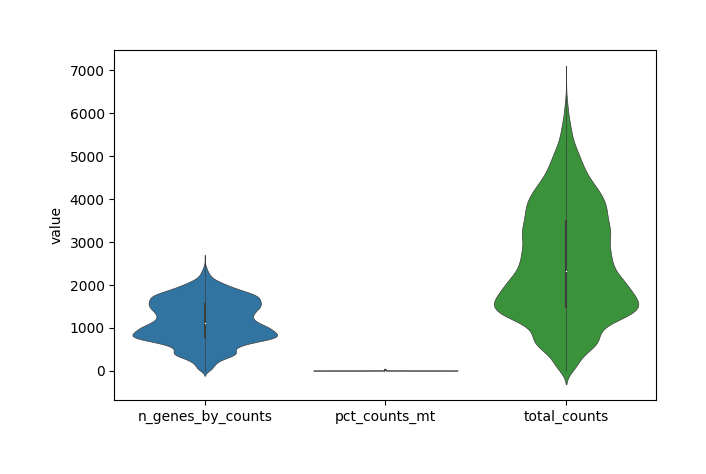
Quality Control
This module calculates the quality distribution of original data, using three indicators:
total_counts - the total counts per cell;

n_genes_by_counts - the number of genes expressed in count maxtrix;

pct_countss_mt - the percentage of counts in mitochondrial genes.
[5]:
data.tl.cal_qc()
[2024-01-17 10:20:01][Stereo][3643][MainThread][140100178437952][st_pipeline][41][INFO]: start to run cal_qc...
[2024-01-17 10:20:01][Stereo][3643][MainThread][140100178437952][st_pipeline][44][INFO]: cal_qc end, consume time 0.4553s.
Show the violin figure of QC distribution.
[6]:
data.plt.violin()
Note
Just input your file name and click the download button to save visualization result, or set parameter in plot functions.
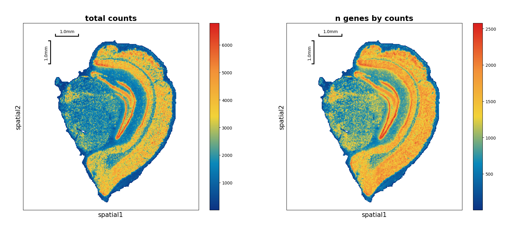
Show the spatial scatter figure of QC distribution.
[7]:
data.plt.spatial_scatter()
[7]:
Filtering
Three basic methods are provided to filter data maxtrix:
data.tl.filter_cells, data.tl.filter_genes, data.tl.filter_coordinates.
Literally, you could filter data on three optional levels: cell, gene and coordinate where a bin unit could be treated as a made-up cell provisionally.
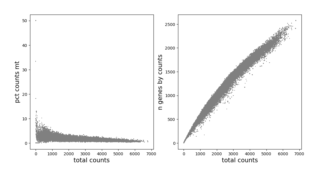
We filter bin units (bin_size is set to 50 at the beginning of our example) based on quality control indicators which have been calculated in QC part. Beforehand, observe the distribution of cells according to scatter plots.
[8]:
data.plt.genes_count()
[8]:
Remove cells that have too many mitochondrial genes expressed, as well as cells without enough counts and genes expressed.
[9]:
data.tl.filter_cells(
        min_counts=20,
        min_genes=3,
        pct_counts_mt=5,
        inplace=True
        )
data
[2024-01-17 10:20:05][Stereo][3643][MainThread][140100178437952][st_pipeline][41][INFO]: start to run filter_cells...
[2024-01-17 10:20:06][Stereo][3643][MainThread][140100178437952][st_pipeline][44][INFO]: filter_cells end, consume time 0.4412s.
[9]:
StereoExpData object with n_cells X n_genes = 35738 X 24302
bin_type: bins
bin_size: 50
offset_x = 0
offset_y = 0
cells: ['cell_name', 'total_counts', 'n_genes_by_counts', 'pct_counts_mt']
genes: ['gene_name', 'n_cells', 'n_counts', 'mean_umi']
result: []
Note
We strongly suggest to use self.raw to record the raw gene expression matrix which has been gone through basic processing, as an essential data set for subsequent differential testing and multiple analysis.
So in order to save the data and recall it conveniently, you can save the raw expression matrix by data.tl.raw_checkpoint().
[10]:
data.tl.raw_checkpoint()
[11]:
data.tl.raw
[11]:
StereoExpData object with n_cells X n_genes = 35738 X 24302
bin_type: bins
bin_size: 50
offset_x = 0
offset_y = 0
cells: ['cell_name', 'total_counts', 'n_genes_by_counts', 'pct_counts_mt']
genes: ['gene_name', 'n_cells', 'n_counts', 'mean_umi']
result: []
Note
When you want to get raw data, just run data.tl.reset_raw_data().
Normalization
In this module, you can choose from following common methods of standardization:
Note
If the parameter inplace is set to True by default, expression matrix data will be replaced by the corresponding result (here replaced by the normalized result), otherwise unchanged.
Run a combination method of normalize_total and log1p to normalize gene expression matrix as below:
[12]:
# inplace is set to True by default

data.tl.normalize_total(target_sum=10000)
data.tl.log1p()
[2024-01-17 10:20:06][Stereo][3643][MainThread][140100178437952][st_pipeline][41][INFO]: start to run normalize_total...
[2024-01-17 10:20:06][Stereo][3643][MainThread][140100178437952][st_pipeline][44][INFO]: normalize_total end, consume time 0.3486s.
[2024-01-17 10:20:06][Stereo][3643][MainThread][140100178437952][st_pipeline][41][INFO]: start to run log1p...
[2024-01-17 10:20:06][Stereo][3643][MainThread][140100178437952][st_pipeline][44][INFO]: log1p end, consume time 0.0977s.
If you use data.tl.sctransform which includes the function of finding highly variable genes, you do not need to run data.tl.highly_variable_genes. In the subsequent data.tl.pca method, the parameter use_highly_genes has to be set as False. In brief, whether to use highly variable genes to run PCA depends on filter_hvgs in the normalization of scTransform. Learn more about
scTransform.
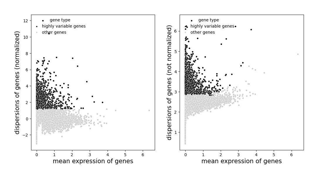
Highly variable genes
Identify highly variable genes in cells.
[13]:
data.tl.highly_variable_genes(
        min_mean=0.0125,
        max_mean=3,
        min_disp=0.5,
        n_top_genes=2000,
        res_key='highly_variable_genes'
        )
[2024-01-17 10:20:06][Stereo][3643][MainThread][140100178437952][st_pipeline][41][INFO]: start to run highly_variable_genes...
[2024-01-17 10:20:07][Stereo][3643][MainThread][140100178437952][st_pipeline][44][INFO]: highly_variable_genes end, consume time 0.7429s.
If data.tl.scale(zero_center=False) is used, sparse matrix will be used for calculation, which can greatly reduce the memory required for running.
[14]:
# remember to choose a res_key when plot

data.plt.highly_variable_genes(res_key='highly_variable_genes')
[14]:
Scale each gene to unit variance. Clip values exceeding standard deviation 10. If data.tl.scale(zero_center=False) is used, sparse matrix will be used for calculation, which can greatly reduce the memory required for running.
[15]:
data.tl.scale(max_value=10, zero_center=True)
[2024-01-17 10:20:09][Stereo][3643][MainThread][140100178437952][st_pipeline][41][INFO]: start to run scale...
[2024-01-17 10:20:17][Stereo][3643][MainThread][140100178437952][scale][53][INFO]: Truncate at max_value 10
[2024-01-17 10:20:17][Stereo][3643][MainThread][140100178437952][st_pipeline][44][INFO]: scale end, consume time 8.3585s.
Embedding
PCA (Principal component analysis)
As a statistical technique for reducing dimensionality of a data set, PCA finds the max axes of greatest variation, which preserve as much information as possible. Notice that if set parameter use_highly_genes to True, only highly variable genes are used to run.
[16]:
data.tl.pca(
        use_highly_genes=False,
        n_pcs=30,
        res_key='pca'
        )
[2024-01-17 10:20:17][Stereo][3643][MainThread][140100178437952][st_pipeline][41][INFO]: start to run pca...
[2024-01-17 10:20:32][Stereo][3643][MainThread][140100178437952][st_pipeline][44][INFO]: pca end, consume time 14.8000s.
When the parameter res_key arises, the corresponding result will be stored automatically, simply check:
[17]:
data.tl.key_record
[17]:
{'hvg': ['highly_variable_genes'],
 'pca': ['pca'],
 'neighbors': [],
 'umap': [],
 'cluster': [],
 'marker_genes': []}
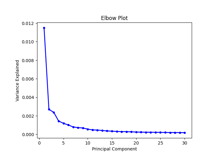
We can plot the elbow to help us to determine how to choose PCs to be used.
[18]:
data.plt.elbow(pca_res_key='pca')
[2024-01-17 10:20:32][Stereo][3643][MainThread][140100178437952][plot_collection][84][INFO]: register plot_func elbow to <stereo.plots.plot_collection.PlotCollection object at 0x7f6b322ce700>
[18]:
Neighborhood graph
After PCA, we compute the neighborhood graph of cells using the PCA representation of the expression matrix.
[19]:
data.tl.neighbors(
        pca_res_key='pca',
        n_pcs=30,
        res_key='neighbors'
        )

# compute spatial neighbors
data.tl.spatial_neighbors(
        neighbors_res_key='neighbors',
        res_key='spatial_neighbors'
        )
[2024-01-17 10:20:33][Stereo][3643][MainThread][140100178437952][st_pipeline][41][INFO]: start to run neighbors...
[2024-01-17 10:20:53][Stereo][3643][MainThread][140100178437952][st_pipeline][44][INFO]: neighbors end, consume time 20.3813s.
[2024-01-17 10:20:53][Stereo][3643][MainThread][140100178437952][st_pipeline][41][INFO]: start to run spatial_neighbors...
[2024-01-17 10:20:57][Stereo][3643][MainThread][140100178437952][reader][821][INFO]: Adding sample in adata.obs['orig.ident'].
[2024-01-17 10:20:57][Stereo][3643][MainThread][140100178437952][reader][824][INFO]: Adding data.position as adata.obsm['spatial'] .
[2024-01-17 10:20:57][Stereo][3643][MainThread][140100178437952][reader][829][INFO]: Adding data.position as adata.obs['x'] and adata.obs['y'] .
[2024-01-17 10:20:58][Stereo][3643][MainThread][140100178437952][reader][859][INFO]: Adding data.tl.result['highly_variable_genes'] into adata.var .
[2024-01-17 10:20:58][Stereo][3643][MainThread][140100178437952][reader][881][INFO]: Adding data.tl.result['pca'] into adata.obsm['X_pca'] .
[2024-01-17 10:20:58][Stereo][3643][MainThread][140100178437952][reader][889][INFO]: Adding data.tl.result['neighbors']['connectivities'] into adata.obsp['connectivities'] .
[2024-01-17 10:20:58][Stereo][3643][MainThread][140100178437952][reader][890][INFO]: Adding data.tl.result['neighbors']['nn_dist'] into adata.obsp['distances'] .
[2024-01-17 10:20:58][Stereo][3643][MainThread][140100178437952][reader][893][INFO]: Adding info into adata.uns['neighbors'].
[2024-01-17 10:20:58][Stereo][3643][MainThread][140100178437952][reader][942][INFO]: Adding data.tl.raw.exp_matrix as adata.raw .
[2024-01-17 10:21:00][Stereo][3643][MainThread][140100178437952][reader][964][INFO]: Finished conversion to anndata.
[2024-01-17 10:21:01][Stereo][3643][MainThread][140100178437952][st_pipeline][44][INFO]: spatial_neighbors end, consume time 7.7638s.
In addition, we also provide data.tl.spatial_neighbors to compute a spatial neighbors graph.
UMAP
It’s strongly to suggest embedding the graph in two dimensions using UMAP.
[20]:
data.tl.umap(pca_res_key='pca', neighbors_res_key='neighbors', res_key='umap')
[2024-01-17 10:21:01][Stereo][3643][MainThread][140100178437952][st_pipeline][41][INFO]: start to run umap...
        completed  0  /  200 epochs
        completed  20  /  200 epochs
        completed  40  /  200 epochs
        completed  60  /  200 epochs
        completed  80  /  200 epochs
        completed  100  /  200 epochs
        completed  120  /  200 epochs
        completed  140  /  200 epochs
        completed  160  /  200 epochs
        completed  180  /  200 epochs
[2024-01-17 10:21:28][Stereo][3643][MainThread][140100178437952][st_pipeline][44][INFO]: umap end, consume time 27.1704s.
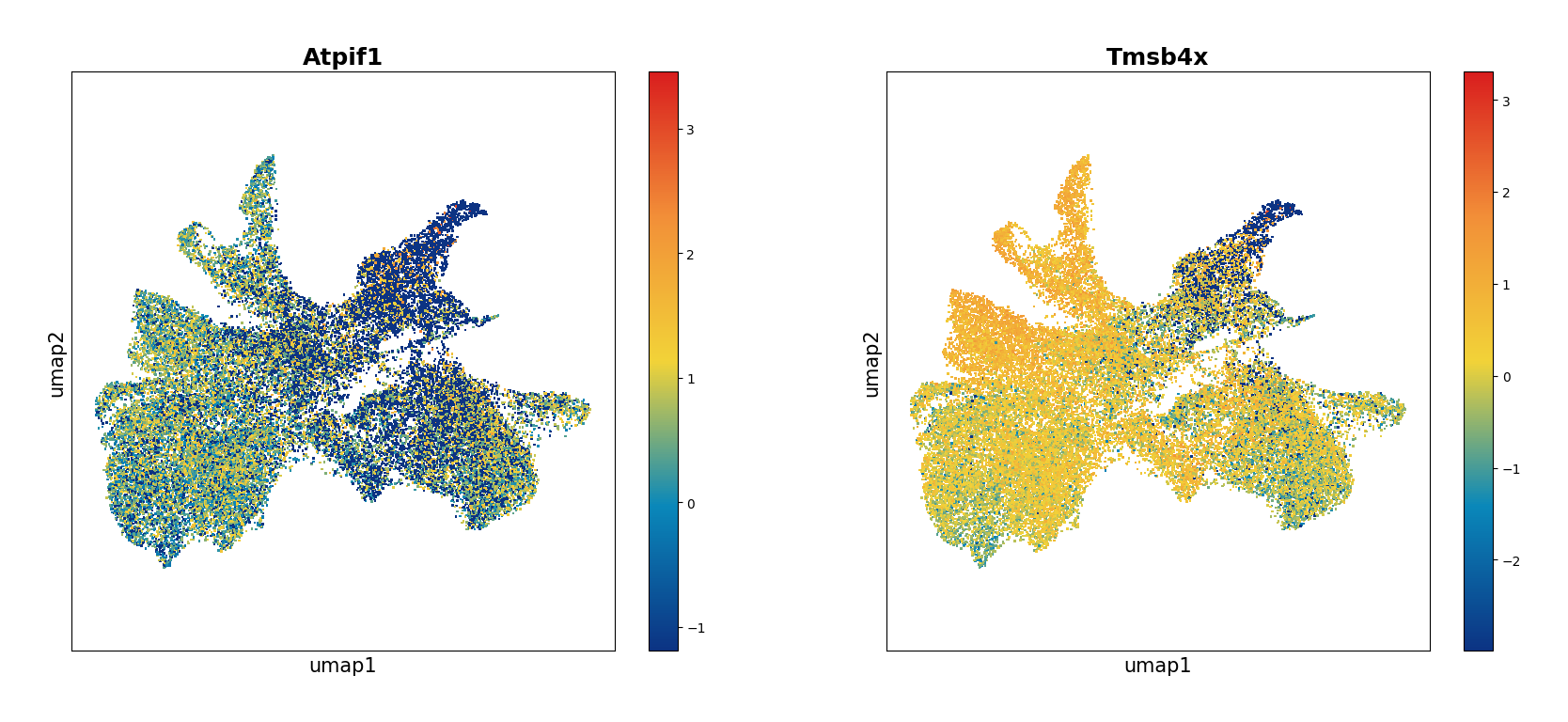
Plot the umap result of two genes: Atpif1 and Tmsb4x.
[21]:
data.plt.umap(gene_names=['Atpif1', 'Tmsb4x'], res_key='umap')
[21]:
Clustering
Currently we provide three common clustering methods, including Leiden, Louvain and Phenograph.
In this tool, you can re-run the normalization method before clustering if the parameter normalize_method is not None. Then by default, we perform PCA to reduce the dimensionalites of the new normalization result, and use top 30 pcs to run clustering.
At this stage, we strongly recommend using leiden.
Leiden
Simply run:
[22]:
data.tl.leiden(neighbors_res_key='neighbors', res_key='leiden')
[2024-01-17 10:22:04][Stereo][3643][MainThread][140100178437952][st_pipeline][41][INFO]: start to run leiden...
[2024-01-17 10:22:27][Stereo][3643][MainThread][140100178437952][st_pipeline][44][INFO]: leiden end, consume time 22.6067s.
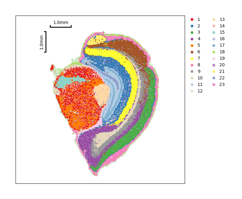
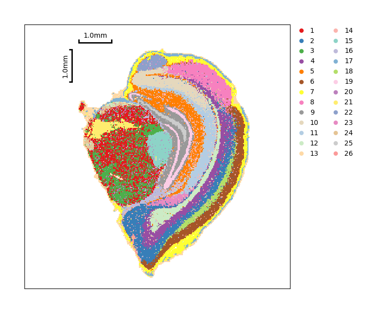
Show the spatial distribution of the Leiden clustering.
[23]:
data.plt.cluster_scatter(res_key='leiden')
[23]:
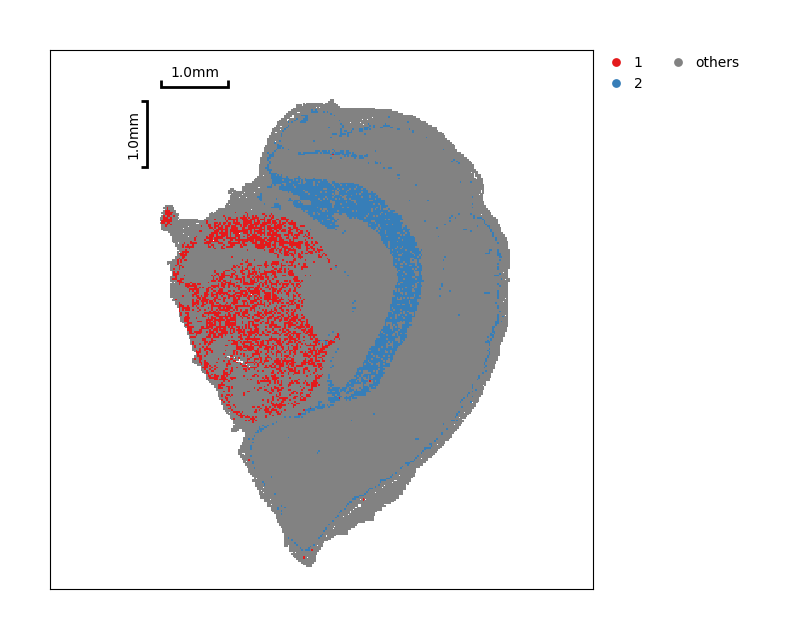
You also can just show partial clustering result.
[24]:
data.plt.cluster_scatter(res_key='leiden', groups=['1', '2'])
[24]:
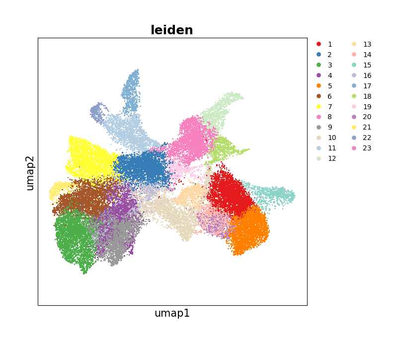
Show the distribution of the UMAP embedding.
[25]:
data.plt.umap(res_key='umap', cluster_key='leiden')
[25]:
data.plt.interact_cluster generates an interact module from Jupyter Notebook and basic interactive manipulations could be done here. Simple clicks help you finish a series of operations, inclusing moving, tailoring, dyeing, saving and etc., over different clustering groups. More about in Interactive cluster.
[26]:
data.plt.interact_cluster(res_key='leiden')
[26]:
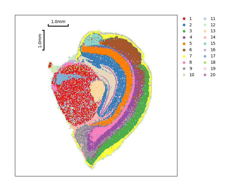
The same way to display results of distribution, using spatial neighbors:
[27]:
data.tl.leiden(neighbors_res_key='spatial_neighbors', res_key='spatial_leiden')
[2024-01-17 10:22:31][Stereo][3643][MainThread][140100178437952][st_pipeline][41][INFO]: start to run leiden...
[2024-01-17 10:22:57][Stereo][3643][MainThread][140100178437952][st_pipeline][44][INFO]: leiden end, consume time 26.4340s.
[28]:
data.plt.cluster_scatter(res_key='spatial_leiden')
[28]:
Louvain
When clustering by Louvain algorithm, just run:
[29]:
data.tl.louvain(neighbors_res_key='neighbors', res_key='louvain')
[2024-01-17 10:22:58][Stereo][3643][MainThread][140100178437952][st_pipeline][41][INFO]: start to run louvain...
[2024-01-17 10:22:58][Stereo][3643][MainThread][140100178437952][_louvain][109][INFO]:     using the "louvain" package of Traag (2017)
[2024-01-17 10:23:02][Stereo][3643][MainThread][140100178437952][st_pipeline][44][INFO]: louvain end, consume time 3.8535s.
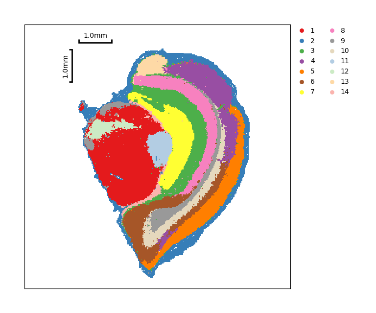
Show the spatial distribution of Louvain clustering.
[30]:
data.plt.cluster_scatter(res_key='louvain')
[30]:
Phenograph
When clustering by Phenograph algorithm, just run:
[31]:
data.tl.phenograph(phenograph_k=30, pca_res_key='pca', res_key='phenograph')
[2024-01-17 10:23:03][Stereo][3643][MainThread][140100178437952][st_pipeline][41][INFO]: start to run phenograph...
Finding 30 nearest neighbors using minkowski metric and 'auto' algorithm
Neighbors computed in 1.8044803142547607 seconds
Jaccard graph constructed in 21.25911808013916 seconds
Running Leiden optimization
Leiden completed in 19.410745859146118 seconds
Sorting communities by size, please wait ...
PhenoGraph completed in 56.2121479511261 seconds
[2024-01-17 10:24:00][Stereo][3643][MainThread][140100178437952][st_pipeline][44][INFO]: phenograph end, consume time 57.1281s.
Show the spatial distribution of Phenograph clustering.
[32]:
data.plt.cluster_scatter(res_key='phenograph')
[32]:
Find Marker Genes
Hypothesis test is used to compute a ranking of differentially expressed genes among clusters. The raw count of express matrix which has been saved in self.raw by data.tl.raw_checkpoint() and highly variable genes are two optional data sets, used to find marker genes.
Here supports two methods, t_test and wilcoxon_test, to find marker genes between pairs among all clusters. T-test is a common and simple approach to do so.
[33]:
data.tl.find_marker_genes(
        cluster_res_key='leiden',
        method='t_test',
        use_highly_genes=False,
        use_raw=True
        )
[2024-01-17 10:24:01][Stereo][3643][MainThread][140100178437952][st_pipeline][41][INFO]: start to run find_marker_genes...
[2024-01-17 10:24:01][Stereo][3643][MainThread][140100178437952][tool_base][122][INFO]: read group information, grouping by group column.
[2024-01-17 10:24:01][Stereo][3643][MainThread][140100178437952][tool_base][151][INFO]: start to run...
[2024-01-17 10:24:01][Stereo][3643][MainThread][140100178437952][time_consume][57][INFO]: start to run calc_pct_and_pct_rest...
[2024-01-17 10:24:03][Stereo][3643][MainThread][140100178437952][time_consume][60][INFO]: calc_pct_and_pct_rest end, consume time 1.8275s.
[2024-01-17 10:24:09][Stereo][3643][MainThread][140100178437952][tool_base][153][INFO]: end to run.
[2024-01-17 10:24:09][Stereo][3643][MainThread][140100178437952][st_pipeline][44][INFO]: find_marker_genes end, consume time 7.7700s.
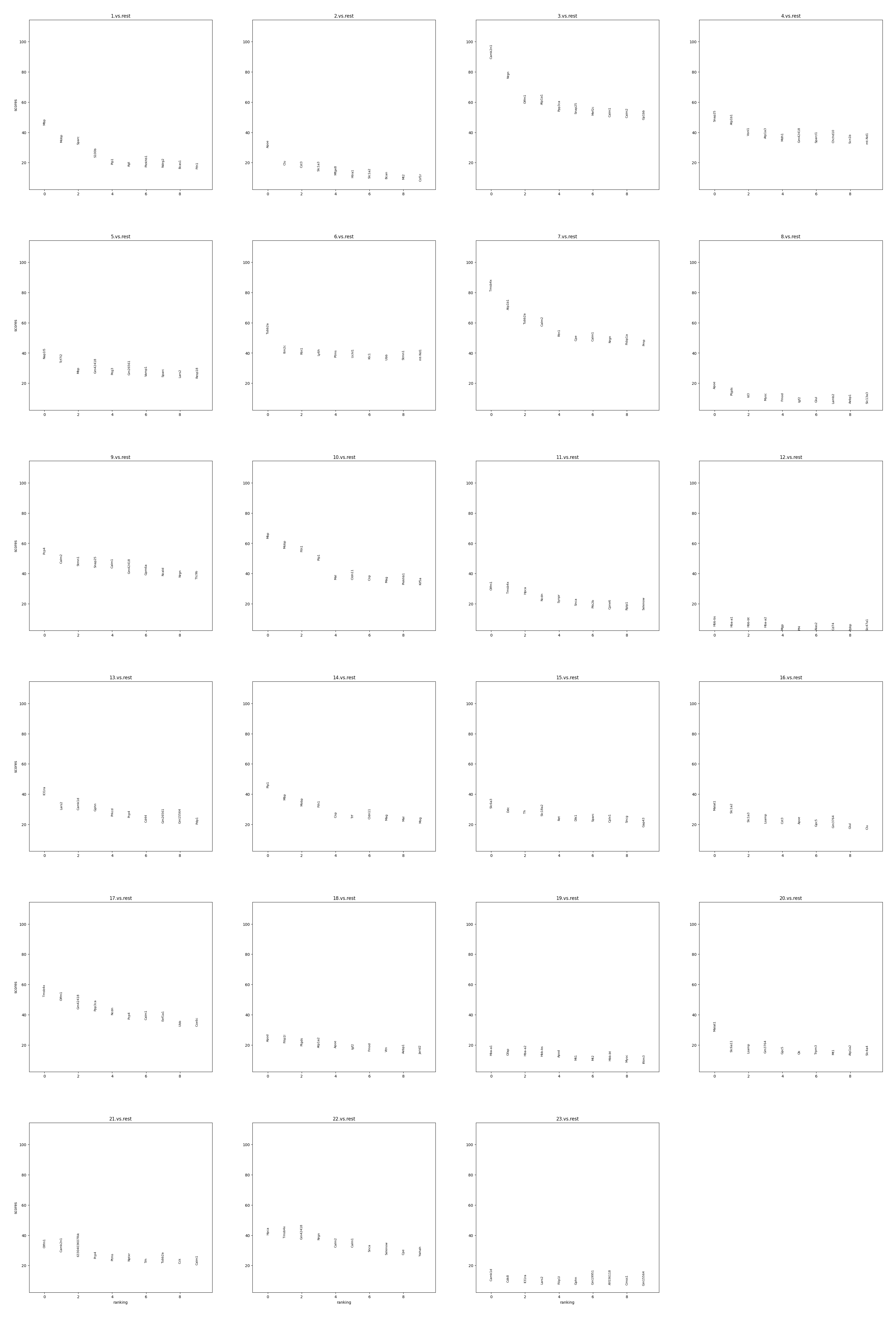
Display the ranking and scores of top 10 marker genes in each group.
[34]:
data.plt.marker_genes_text(
        res_key='marker_genes',
        markers_num=10,
        sort_key='scores'
        )
[34]:
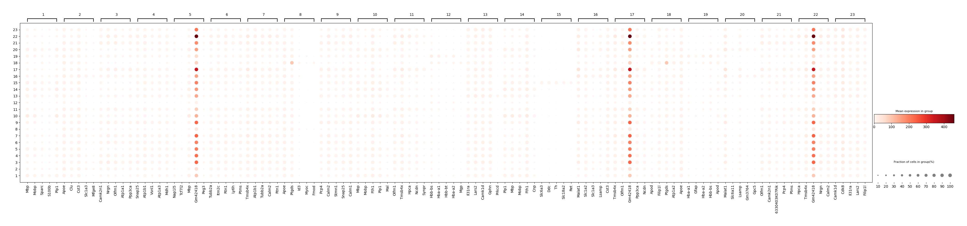
Display the scatter plot of top 5 marker genes in each group.
[35]:
data.plt.marker_genes_scatter(res_key='marker_genes', markers_num=5)
[35]:
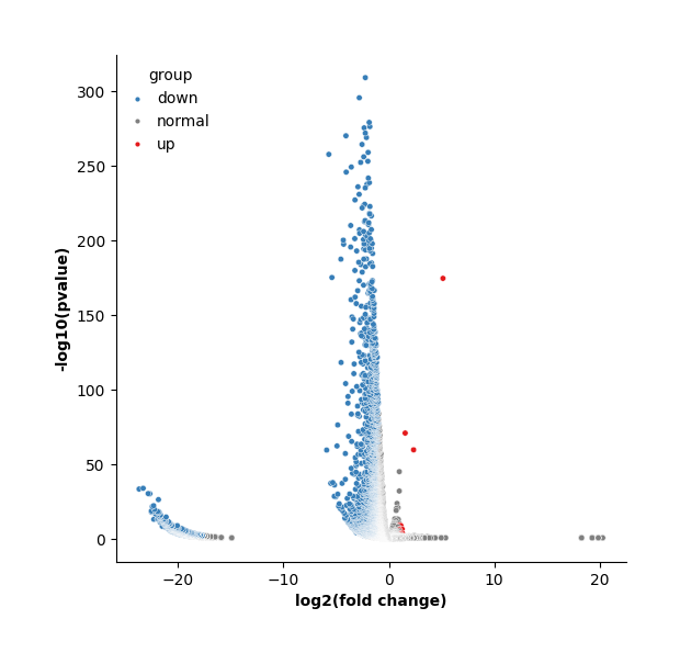
Meanwhile, display the volcano plot of a specific group versus to the rest.
[36]:
data.plt.marker_gene_volcano(group_name='2.vs.rest', vlines=False)
[36]:
You can also filter out genes based on log fold change and fraction of genes expressing the gene within and outside each group.
[37]:
data.tl.filter_marker_genes(
    marker_genes_res_key='marker_genes',
    min_fold_change=1,
    min_in_group_fraction=0.25,
    max_out_group_fraction=0.5,
    res_key='marker_genes_filtered'
)
[2024-01-17 10:24:35][Stereo][3643][MainThread][140100178437952][st_pipeline][41][INFO]: start to run filter_marker_genes...
[2024-01-17 10:24:36][Stereo][3643][MainThread][140100178437952][st_pipeline][44][INFO]: filter_marker_genes end, consume time 1.0848s.
Annotation
After finding marker genes, we can annotate clustering results by using data.tl.annotation or data.plt.interact_annotation_cluster.
[38]:
data.plt.interact_annotation_cluster(
            res_cluster_key='leiden',
            res_marker_gene_key='marker_genes',
            res_key='leiden_annotation'
            )
[38]:
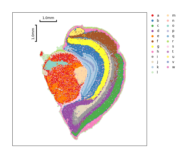
Use command lines to annotate clusters:
[39]:
annotation_dict = {
    '1':'a', '2':'b',
    '3':'c', '4':'d',
    '5':'e', '6':'f',
    '7':'g', '8':'h',
    '9':'i', '10':'j',
    '11':'k', '12': 'l',
    '13': 'm', '14': 'n',
    '15': 'o', '16': 'p',
    '17': 'q', '18': 'r',
    '19': 's', '20': 't',
    '21': 'u', '22': 'v',
    '23': 'w', '24': 'x',
    '25': 'y', '26': 'z'
    }
data.tl.annotation(
        annotation_information=annotation_dict,
        cluster_res_key='leiden',
        res_key='anno_leiden'
        )
[2024-01-17 10:24:38][Stereo][3643][MainThread][140100178437952][st_pipeline][41][INFO]: start to run annotation...
[2024-01-17 10:24:38][Stereo][3643][MainThread][140100178437952][st_pipeline][44][INFO]: annotation end, consume time 0.8266s.
[40]:
data.plt.cluster_scatter(res_key='anno_leiden')
[40]:
At the end, you could transform our data object to AnnData and save analysis results into an H5ad file.
[47]:
adata = st.io.stereo_to_anndata(data, output='SS200000135TL_D1_seurat.h5ad')
[2024-01-17 10:29:45][Stereo][3643][MainThread][140100178437952][reader][821][INFO]: Adding sample in adata.obs['orig.ident'].
[2024-01-17 10:29:45][Stereo][3643][MainThread][140100178437952][reader][824][INFO]: Adding data.position as adata.obsm['spatial'] .
[2024-01-17 10:29:45][Stereo][3643][MainThread][140100178437952][reader][829][INFO]: Adding data.position as adata.obs['x'] and adata.obs['y'] .
[2024-01-17 10:29:45][Stereo][3643][MainThread][140100178437952][reader][859][INFO]: Adding data.tl.result['highly_variable_genes'] into adata.var .
[2024-01-17 10:29:45][Stereo][3643][MainThread][140100178437952][reader][881][INFO]: Adding data.tl.result['pca'] into adata.obsm['X_pca'] .
[2024-01-17 10:29:45][Stereo][3643][MainThread][140100178437952][reader][889][INFO]: Adding data.tl.result['neighbors']['connectivities'] into adata.obsp['connectivities'] .
[2024-01-17 10:29:45][Stereo][3643][MainThread][140100178437952][reader][890][INFO]: Adding data.tl.result['neighbors']['nn_dist'] into adata.obsp['distances'] .
[2024-01-17 10:29:45][Stereo][3643][MainThread][140100178437952][reader][893][INFO]: Adding info into adata.uns['neighbors'].
[2024-01-17 10:29:45][Stereo][3643][MainThread][140100178437952][reader][889][INFO]: Adding data.tl.result['spatial_neighbors']['connectivities'] into adata.obsp['spatial_neighbors_connectivities'] .
[2024-01-17 10:29:45][Stereo][3643][MainThread][140100178437952][reader][890][INFO]: Adding data.tl.result['spatial_neighbors']['nn_dist'] into adata.obsp['spatial_neighbors_distances'] .
[2024-01-17 10:29:45][Stereo][3643][MainThread][140100178437952][reader][893][INFO]: Adding info into adata.uns['spatial_neighbors'].
[2024-01-17 10:29:45][Stereo][3643][MainThread][140100178437952][reader][881][INFO]: Adding data.tl.result['umap'] into adata.obsm['X_umap'] .
[2024-01-17 10:29:45][Stereo][3643][MainThread][140100178437952][reader][900][INFO]: Adding data.tl.result['leiden'] into adata.obs['leiden'] .
[2024-01-17 10:29:45][Stereo][3643][MainThread][140100178437952][reader][900][INFO]: Adding data.tl.result['spatial_leiden'] into adata.obs['spatial_leiden'] .
[2024-01-17 10:29:45][Stereo][3643][MainThread][140100178437952][reader][900][INFO]: Adding data.tl.result['louvain'] into adata.obs['louvain'] .
[2024-01-17 10:29:45][Stereo][3643][MainThread][140100178437952][reader][900][INFO]: Adding data.tl.result['phenograph'] into adata.obs['phenograph'] .
[2024-01-17 10:29:45][Stereo][3643][MainThread][140100178437952][reader][900][INFO]: Adding data.tl.result['anno_leiden'] into adata.obs['anno_leiden'] .
[2024-01-17 10:29:45][Stereo][3643][MainThread][140100178437952][reader][906][INFO]: Adding data.tl.result['gene_exp_leiden'] into adata.uns['gene_exp_leiden']
[2024-01-17 10:29:45][Stereo][3643][MainThread][140100178437952][reader][906][INFO]: Adding data.tl.result['gene_exp_spatial_leiden'] into adata.uns['gene_exp_spatial_leiden']
[2024-01-17 10:29:45][Stereo][3643][MainThread][140100178437952][reader][906][INFO]: Adding data.tl.result['gene_exp_louvain'] into adata.uns['gene_exp_louvain']
[2024-01-17 10:29:45][Stereo][3643][MainThread][140100178437952][reader][906][INFO]: Adding data.tl.result['gene_exp_phenograph'] into adata.uns['gene_exp_phenograph']
[2024-01-17 10:29:45][Stereo][3643][MainThread][140100178437952][reader][906][INFO]: Adding data.tl.result['gene_exp_anno_leiden'] into adata.uns['gene_exp_anno_leiden']
[2024-01-17 10:29:45][Stereo][3643][MainThread][140100178437952][reader][942][INFO]: Adding data.tl.raw.exp_matrix as adata.raw .
[2024-01-17 10:29:47][Stereo][3643][MainThread][140100178437952][reader][964][INFO]: Finished conversion to anndata.
... storing 'gene type' as categorical
[2024-01-17 10:30:05][Stereo][3643][MainThread][140100178437952][reader][968][INFO]: Finished output to SS200000135TL_D1_seurat.h5ad
[48]:
adata
[48]:
AnnData object with n_obs × n_vars = 35738 × 24302
    obs: 'total_counts', 'n_genes_by_counts', 'pct_counts_mt', 'leiden', 'spatial_leiden', 'louvain', 'phenograph', 'anno_leiden', 'orig.ident', 'x', 'y'
    var: 'n_cells', 'n_counts', 'mean_umi', 'hvgs', 'means', 'dispersions', 'dispersions_norm', 'highly_variable', 'gene type'
    uns: 'bin_type', 'bin_size', 'resolution', 'sn', 'hvg', 'neighbors', 'spatial_neighbors', 'gene_exp_leiden', 'gene_exp_spatial_leiden', 'gene_exp_louvain', 'gene_exp_phenograph', 'gene_exp_anno_leiden'
    obsm: 'spatial', 'X_pca', 'X_umap'
    obsp: 'connectivities', 'distances', 'spatial_neighbors_connectivities', 'spatial_neighbors_distances'