Cell-Cell Communication
Cell-cell communication (CCC) refers to the process by which cells interact with each other, using molecular signals. The signals can be transmitted through various mechanisms, such as the release of signaling molecules called ligands by one cell that bind to receptors on another cell, or through direct physical contact between cells. CCC plays a critical role in a wide range of biological processes, including development, immune responses, and tissue repair, among others. In this section, we will provide a concise overview of the process for conducting CCC analysis using Stereopy.
Cell clustering
Download our example data, and complete basic analysis processing.
[1]:
import stereo as st
import warnings
warnings.filterwarnings('ignore')


Before proceeding with the cell-cell communication analysis, make sure to perform the necessary cell clustering analysis if it hasn’t been completed yet.
[2]:
data = st.io.read_h5ad('../test_data/mouse_embryo_heart_new.h5ad')
# preprocessing
data.tl.cal_qc()
# data.plt.genes_count is a good option to observe gene distribution before filtering
# data.tl.filter_cells(min_counts=1, max_counts=2000, min_genes=3, max_genes=800, pct_counts_mt=6, inplace=True)
data.tl.raw_checkpoint()
data.tl.normalize_total()
# clustering
data.tl.pca(n_pcs=50, res_key='pca', use_highly_genes=False)
data.tl.neighbors(pca_res_key='pca', res_key='neighbors')
data.tl.leiden(neighbors_res_key='neighbors', res_key='leiden')
# data.plt.cluster_scatter(res_key='leiden', plotting_scale_width=2)
[2023-11-15 11:35:58][Stereo][21850][MainThread][139852866279232][st_pipeline][41][INFO]: start to run cal_qc...
[2023-11-15 11:35:59][Stereo][21850][MainThread][139852866279232][st_pipeline][44][INFO]: cal_qc end, consume time 0.5781s.
[2023-11-15 11:35:59][Stereo][21850][MainThread][139852866279232][st_pipeline][41][INFO]: start to run normalize_total...
[2023-11-15 11:35:59][Stereo][21850][MainThread][139852866279232][st_pipeline][44][INFO]: normalize_total end, consume time 0.2943s.
[2023-11-15 11:35:59][Stereo][21850][MainThread][139852866279232][st_pipeline][41][INFO]: start to run pca...
[2023-11-15 11:35:59][Stereo][21850][MainThread][139852866279232][dim_reduce][78][WARNING]: svd_solver: auto can not be used with sparse input.
Use "arpack" (the default) instead.
[2023-11-15 11:36:34][Stereo][21850][MainThread][139852866279232][st_pipeline][44][INFO]: pca end, consume time 34.5284s.
[2023-11-15 11:36:34][Stereo][21850][MainThread][139852866279232][st_pipeline][41][INFO]: start to run neighbors...
[2023-11-15 11:40:43][Stereo][21850][MainThread][139852866279232][st_pipeline][44][INFO]: neighbors end, consume time 249.7218s.
[2023-11-15 11:40:43][Stereo][21850][MainThread][139852866279232][st_pipeline][41][INFO]: start to run leiden...
[2023-11-15 11:41:10][Stereo][21850][MainThread][139852866279232][st_pipeline][44][INFO]: leiden end, consume time 26.3186s.
Note
Since this example data already have cell type labels stored in obs, we can omit the clustering step and proceed directly to the next section.
[3]:
data.plt.cluster_scatter(res_key='celltype', show_plotting_scale=False)
[3]:

Spatial information incorperation
To incorperate the spatial information and ensure the accuracy of the signaling model, we assume that intercellular ligand-receptor (L-R) communications routinely exist among closely neighboring cells.
Before conducting the communication analysis, it is advisable to filter the cells that are located in close proximity to each other. This step ensures that the cells considered for communication analysis are physically close enough to facilitate actual communication. Nevertheless, you can always skip this step and proceed directly to the actual CCC analysis part using the entire dataset.
In Stereopy, we provide two approaches for performing spatial filteration.
Microenvironment
The first step is input microenvironment information into the communication analysis. It treats each cell type as a cohesive unit, and microenvironments are formed by combining two or more closely located cell types. Microenvironments can be calculated with data.tl.gen_ccc_micro_envs. We provide two approaches when calculating microenvironments: one is using the minimum spanning tree (MST); the other is through splitting the fully connected network into multiple strongly connected
components.
This function should be ran twice because it includes two parts:
Calculating how clusters are divided into microenvironments under diffrent thresholds.
Generating microenvironments by choosing an appropriate
methodandthresholdbased on the result of first part.
More details refer to API.
[4]:
data.tl.gen_ccc_micro_envs(
cluster_res_key='celltype',
res_key='ccc_micro_envs'
)
[2023-11-15 11:41:14][Stereo][21850][MainThread][139852866279232][st_pipeline][77][INFO]: register algorithm gen_ccc_micro_envs to <stereo.core.st_pipeline.AnnBasedStPipeline object at 0x7f31b4323340>
Now, you can choose a appropriate threshold based on this function's result.
[4]:
Note
The coordinates must be stored as x and y in obs, or spatial in obsm.
The final bootstrap MST is stored in mst_final and pairwise KL-divergences are stored in pairwise_kl_divergence of uns['ccc_micro_envs']. Pick a proper method and threshold to get the final microenvironments.
[5]:
data.tl.gen_ccc_micro_envs(
method='split',
threshold=2,
res_key='ccc_micro_envs'
)
Using the ‘split’ method with theshold 2, we got two microenvironments as follows:
[6]:
data.tl.result['ccc_micro_envs']['micro_envs']
[6]:
| cell_type | microenvironment | |
|---|---|---|
| 0 | endocardial/endothelial (EC) | microenv_0 |
| 1 | ventricular-specific CM | microenv_0 |
| 2 | atrial-specific CM | microenv_0 |
| 3 | epicardial (EP) | microenv_0 |
| 4 | blood | microenv_1 |
| 5 | fibro-mesenchymal (FM) | microenv_1 |
Niche
The alternative filteration approach constructs a niche for two given cell types at individual cell level. For each cell of type 1, only cells of type 2 that are within a certain Euclidean distance threshold, denoted as niche_distance, are retained. The niche of cell type 1 and 2 is constructed by including all cells of type 1 that have type 2 neighbors, as well as all their neighboring type 2 cells.
You can run data.tl.get_niche to get a new data object based on a pair of cell clusters, which represents a niche.
Afterwards, run communication analysis based on this niche.
More in API.
[7]:
data_niche = data.tl.get_niche(
niche_distance=0.025,
cluster_1='epicardial (EP)',
cluster_2='ventricular-specific CM',
cluster_res_key='celltype'
)
data_niche
[2023-11-15 11:41:21][Stereo][21850][MainThread][139852866279232][st_pipeline][77][INFO]: register algorithm get_niche to <stereo.core.st_pipeline.AnnBasedStPipeline object at 0x7f31b4323340>
[7]:
AnnData object with n_obs × n_vars = 14792 × 30254
obs: 'ctype_user', 'slice', 'seurat_clusters', 'celltype', 'DBSCAN', 'total_counts', 'n_genes_by_counts', 'pct_counts_mt', 'leiden'
var: 'n_cells', 'n_counts', 'mean_umi'
uns: 'sn', 'pca', 'pca_variance_ratio', 'neighbors', 'leiden', 'gene_exp_leiden', 'ccc_micro_envs'
obsm: 'spatial', 'spatial_regis', 'X_pca'
obsp: 'connectivities', 'distances'
Communication analysis
We suggest using normalized non-log-transformed data to do the analysis.
analysis_type can be set to simple or statistical. simple does not rely on any statistics and only provides the mean expression values for each interaction for each possible cell type pair, while statistical also estimates the statistical significance of these mean expression values using a permutation approach.
This function currently supports the species of HUMAN and MOUSE. If input the data of other species, you have to translate the genes to homologous genes of human or mouse. Then select a database from cellphonedb, liana and celltalkdb [Efremova20], or input the path of your own database.
Note
HUMAN species can not be used with celltalkdb database for the moment.
You can incorperate the spatial information by specifying microenvironments with parameter micro_envs:
[8]:
data.tl.cell_cell_communication(
analysis_type='statistical',
cluster_res_key='celltype',
species='MOUSE',
database='liana',
micro_envs='ccc_micro_envs',
res_key='cell_cell_communication'
)
[2023-11-15 11:41:38][Stereo][21850][MainThread][139852866279232][st_pipeline][77][INFO]: register algorithm cell_cell_communication to <stereo.core.st_pipeline.AnnBasedStPipeline object at 0x7f31b4323340>
[2023-11-15 11:41:38][Stereo][21850][MainThread][139852866279232][main][128][INFO]: species: MOUSE
[2023-11-15 11:41:38][Stereo][21850][MainThread][139852866279232][main][129][INFO]: database: liana
[2023-11-15 11:43:06][Stereo][21850][MainThread][139852866279232][main][188][INFO]: [statistical analysis] Threshold:0.1 Precision:3 Iterations:500 Threads:1
[2023-11-15 11:43:29][Stereo][21850][MainThread][139852866279232][main][218][INFO]: Running Real Analysis
[2023-11-15 11:43:29][Stereo][21850][MainThread][139852866279232][main][761][INFO]: Limiting cluster combinations using microenvironments
[2023-11-15 11:43:29][Stereo][21850][MainThread][139852866279232][main][232][INFO]: Running Statistical Analysis
statistical analysis: 100%|███████████████████████████████████████| 500/500 [26:45<00:00, 3.21s/it]
[2023-11-15 12:10:14][Stereo][21850][MainThread][139852866279232][main][1029][INFO]: Building Pvalues result
[2023-11-15 12:10:15][Stereo][21850][MainThread][139852866279232][main][1064][INFO]: Building results
Or directly perform the analysis on the niche StereoExpData:
[9]:
data_niche.tl.cell_cell_communication(
analysis_type='statistical',
cluster_res_key='celltype',
species='MOUSE',
database='liana',
threshold=0.1,
res_key='cell_cell_communication'
)
[2023-11-15 12:10:22][Stereo][21850][MainThread][139852866279232][st_pipeline][77][INFO]: register algorithm cell_cell_communication to <stereo.core.st_pipeline.AnnBasedStPipeline object at 0x7f2ff4f46160>
[2023-11-15 12:10:22][Stereo][21850][MainThread][139852866279232][main][128][INFO]: species: MOUSE
[2023-11-15 12:10:22][Stereo][21850][MainThread][139852866279232][main][129][INFO]: database: liana
[2023-11-15 12:10:36][Stereo][21850][MainThread][139852866279232][main][188][INFO]: [statistical analysis] Threshold:0.1 Precision:3 Iterations:500 Threads:1
[2023-11-15 12:10:40][Stereo][21850][MainThread][139852866279232][main][218][INFO]: Running Real Analysis
[2023-11-15 12:10:40][Stereo][21850][MainThread][139852866279232][main][232][INFO]: Running Statistical Analysis
statistical analysis: 100%|███████████████████████████████████████| 500/500 [04:35<00:00, 1.81it/s]
[2023-11-15 12:15:16][Stereo][21850][MainThread][139852866279232][main][1029][INFO]: Building Pvalues result
[2023-11-15 12:15:16][Stereo][21850][MainThread][139852866279232][main][1064][INFO]: Building results
You could also set subsampling=True to enable subsampling of the cells for faster performance.
Result observation
The results of cell-cell communication are stored in data.tl.result.
The means result shows the mean expression values of each L-R pair for each cell cluster pair.
[10]:
# mean
data_niche.tl.result['cell_cell_communication']['means']
[10]:
| id_cp_interaction | interacting_pair | partner_a | partner_b | gene_a | gene_b | secreted | receptor_a | receptor_b | annotation_strategy | is_integrin | epicardial (EP)|epicardial (EP) | epicardial (EP)|ventricular-specific CM | ventricular-specific CM|epicardial (EP) | ventricular-specific CM|ventricular-specific CM | |
|---|---|---|---|---|---|---|---|---|---|---|---|---|---|---|---|
| 1 | CPI-SS0A7B487D4 | KLRG2_WNT11 | simple:A4D1S0 | simple:O96014 | KLRG2 | WNT11 | False | False | False | user_curated | False | 0.000 | 0.000 | 0.130 | 0.036 |
| 2 | CPI-SS0C08F5056 | FZD9_WNT11 | simple:O00144 | simple:O96014 | FZD9 | WNT11 | False | False | False | user_curated | False | 0.136 | 0.042 | 0.143 | 0.050 |
| 3 | CPI-SS029839DC3 | MUSK_WNT11 | simple:O15146 | simple:O96014 | MUSK | WNT11 | False | False | False | user_curated | False | 0.000 | 0.000 | 0.129 | 0.036 |
| 4 | CPI-SS0F653A282 | FZD6_WNT11 | simple:O60353 | simple:O96014 | FZD6 | WNT11 | False | False | False | user_curated | False | 0.156 | 0.063 | 0.153 | 0.060 |
| 5 | CPI-SS070E5DE9E | FZD7_WNT11 | simple:O75084 | simple:O96014 | FZD7 | WNT11 | False | False | False | user_curated | False | 0.265 | 0.172 | 0.197 | 0.104 |
| ... | ... | ... | ... | ... | ... | ... | ... | ... | ... | ... | ... | ... | ... | ... | ... |
| 4675 | CPI-SS0AEC3600B | NTNG2_LRRC4C | simple:Q96CW9 | simple:Q9HCJ2 | NTNG2 | LRRC4C | False | False | False | user_curated | False | 0.063 | 0.061 | 0.053 | 0.051 |
| 4677 | CPI-SS0F2FBF1F6 | ROBO3_NELL2 | simple:Q96MS0 | simple:Q99435 | ROBO3 | NELL2 | False | False | False | user_curated | False | 0.094 | 0.113 | 0.105 | 0.124 |
| 4678 | CPI-SS0777989FE | DCBLD2_SEMA4B | simple:Q96PD2 | simple:Q9NPR2 | DCBLD2 | SEMA4B | False | False | False | user_curated | False | 0.611 | 0.619 | 0.497 | 0.506 |
| 4681 | CPI-SS0F30C777C | LRRC4C_NTNG1 | simple:Q9HCJ2 | simple:Q9Y2I2 | LRRC4C | NTNG1 | False | False | False | user_curated | False | 0.057 | 0.063 | 0.055 | 0.060 |
| 4682 | CPI-SS0F0C92F50 | RTN4_TNFRSF19 | simple:Q9NQC3 | simple:Q9NS68 | RTN4 | TNFRSF19 | False | False | False | user_curated | False | 1.697 | 1.683 | 1.435 | 1.421 |
3225 rows × 15 columns
If done statistical analysis, the significant_means results only keeps statistical significant mean values in the mean result (non-significant means have a value of -1).
[11]:
# significant mean
data_niche.tl.result['cell_cell_communication']['significant_means'].iloc[:10]
[11]:
| id_cp_interaction | interacting_pair | partner_a | partner_b | gene_a | gene_b | secreted | receptor_a | receptor_b | annotation_strategy | is_integrin | rank | epicardial (EP)|epicardial (EP) | epicardial (EP)|ventricular-specific CM | ventricular-specific CM|epicardial (EP) | ventricular-specific CM|ventricular-specific CM | |
|---|---|---|---|---|---|---|---|---|---|---|---|---|---|---|---|---|
| 507 | CPI-SS020F28ACA | PKM_CD44 | simple:P14618 | simple:P16070 | PKM | CD44 | False | False | False | user_curated | False | 0.25 | -1.000000 | -1.000 | -1.000 | 25.476999 |
| 505 | CPI-SS010B52BDD | VCAN_CD44 | simple:P13611 | simple:P16070 | VCAN | CD44 | False | False | False | user_curated | False | 0.25 | -1.000000 | -1.000 | -1.000 | 20.889999 |
| 3051 | CPI-SS048D2A753 | APP_RPSA | simple:P05067 | simple:P08865 | APP | RPSA | False | False | False | user_curated | False | 0.25 | 13.528000 | -1.000 | -1.000 | -1.000000 |
| 1344 | CPI-SS0375E45FC | DCN_ERBB4 | simple:P07585 | simple:Q15303 | DCN | ERBB4 | False | False | False | user_curated | False | 0.25 | -1.000000 | 3.890 | -1.000 | -1.000000 |
| 2940 | CPI-SS042A6F835 | IGF2_IGF2R | simple:P01344 | simple:P11717 | IGF2 | IGF2R | False | False | False | user_curated | False | 0.50 | 12.075000 | 12.825 | -1.000 | -1.000000 |
| 3944 | CPI-SS016BE33C2 | NCL_PTN | simple:P19338 | simple:P21246 | NCL | PTN | False | False | False | user_curated | False | 0.50 | 9.104000 | -1.000 | 8.968 | -1.000000 |
| 497 | CPI-SS0BCAB7F53 | VIM_CD44 | simple:P08670 | simple:P16070 | VIM | CD44 | False | False | False | user_curated | False | 0.50 | 24.686001 | 25.083 | -1.000 | -1.000000 |
| 495 | CPI-SS0EF14F3FB | COL1A2_CD44 | simple:P08123 | simple:P16070 | COL1A2 | CD44 | False | False | False | user_curated | False | 0.50 | 22.490999 | 22.888 | -1.000 | -1.000000 |
| 1951 | CPI-SS052990001 | ITGB1_VCAN | simple:P05556 | simple:P13611 | ITGB1 | VCAN | False | False | False | user_curated | False | 0.50 | -1.000000 | 3.159 | -1.000 | 2.908000 |
| 490 | CPI-SS0EAB0009F | FN1_CD44 | simple:P02751 | simple:P16070 | FN1 | CD44 | False | False | False | user_curated | False | 0.50 | 24.709999 | 25.107 | -1.000 | -1.000000 |
The pvalues result shows the p-values for each mean value in the means result.
[12]:
# p-value
data_niche.tl.result['cell_cell_communication']['pvalues']
[12]:
| id_cp_interaction | interacting_pair | partner_a | partner_b | gene_a | gene_b | secreted | receptor_a | receptor_b | annotation_strategy | is_integrin | epicardial (EP)|epicardial (EP) | epicardial (EP)|ventricular-specific CM | ventricular-specific CM|epicardial (EP) | ventricular-specific CM|ventricular-specific CM | |
|---|---|---|---|---|---|---|---|---|---|---|---|---|---|---|---|
| 1 | CPI-SS0A7B487D4 | KLRG2_WNT11 | simple:A4D1S0 | simple:O96014 | KLRG2 | WNT11 | False | False | False | user_curated | False | 1.0 | 1.0 | 1.0 | 1.0 |
| 2 | CPI-SS0C08F5056 | FZD9_WNT11 | simple:O00144 | simple:O96014 | FZD9 | WNT11 | False | False | False | user_curated | False | 1.0 | 1.0 | 1.0 | 1.0 |
| 3 | CPI-SS029839DC3 | MUSK_WNT11 | simple:O15146 | simple:O96014 | MUSK | WNT11 | False | False | False | user_curated | False | 1.0 | 1.0 | 1.0 | 1.0 |
| 4 | CPI-SS0F653A282 | FZD6_WNT11 | simple:O60353 | simple:O96014 | FZD6 | WNT11 | False | False | False | user_curated | False | 1.0 | 1.0 | 1.0 | 1.0 |
| 5 | CPI-SS070E5DE9E | FZD7_WNT11 | simple:O75084 | simple:O96014 | FZD7 | WNT11 | False | False | False | user_curated | False | 1.0 | 1.0 | 1.0 | 1.0 |
| ... | ... | ... | ... | ... | ... | ... | ... | ... | ... | ... | ... | ... | ... | ... | ... |
| 4675 | CPI-SS0AEC3600B | NTNG2_LRRC4C | simple:Q96CW9 | simple:Q9HCJ2 | NTNG2 | LRRC4C | False | False | False | user_curated | False | 1.0 | 1.0 | 1.0 | 1.0 |
| 4677 | CPI-SS0F2FBF1F6 | ROBO3_NELL2 | simple:Q96MS0 | simple:Q99435 | ROBO3 | NELL2 | False | False | False | user_curated | False | 1.0 | 1.0 | 1.0 | 1.0 |
| 4678 | CPI-SS0777989FE | DCBLD2_SEMA4B | simple:Q96PD2 | simple:Q9NPR2 | DCBLD2 | SEMA4B | False | False | False | user_curated | False | 1.0 | 1.0 | 1.0 | 1.0 |
| 4681 | CPI-SS0F30C777C | LRRC4C_NTNG1 | simple:Q9HCJ2 | simple:Q9Y2I2 | LRRC4C | NTNG1 | False | False | False | user_curated | False | 1.0 | 1.0 | 1.0 | 1.0 |
| 4682 | CPI-SS0F0C92F50 | RTN4_TNFRSF19 | simple:Q9NQC3 | simple:Q9NS68 | RTN4 | TNFRSF19 | False | False | False | user_curated | False | 1.0 | 1.0 | 1.0 | 1.0 |
3225 rows × 15 columns
Set parameters, output, *_filename and output_format, to save results into files, more in API.
Visualization of communication
We provide dot plot, heatmap, circos plot and sankey plot for visualizing the CCC analysis results.
Note
Currently, only statistical analysis type is supported to visualization.
Note
On this example, you need to replace data_niche to data when running the visualization functions if analysis is done on entire data.
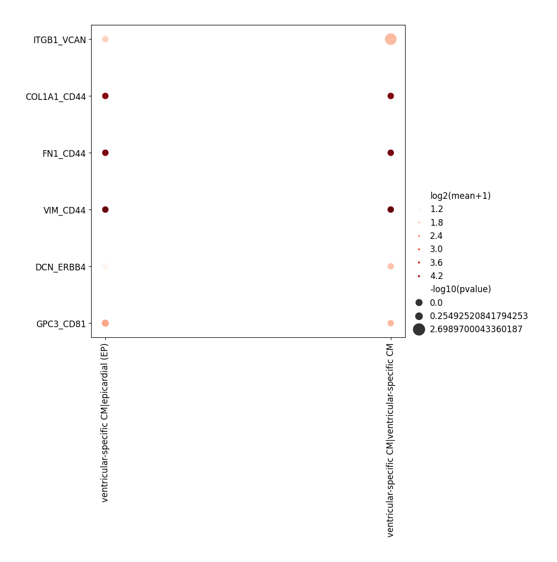
Dotplot
Here we recommend setting interacting_pairs and clusters1 /clusters2 before plotting, because the whole result might be too huge to be displayed.
[13]:
# a list of 'gene1_gene2'
interacting_pairs = [
'GPC3_CD81',
'COL1A1_CD44',
'FN1_CD44',
'DCN_ERBB4',
'VIM_CD44',
'ITGB1_VCAN'
]
# interacting_pairs = None
data_niche.plt.ccc_dot_plot(
res_key='cell_cell_communication',
interacting_pairs=interacting_pairs,
clusters1='ventricular-specific CM'
)
[2023-11-15 12:15:18][Stereo][21850][MainThread][139852866279232][plot_collection][82][INFO]: register plot_func ccc_dot_plot to <stereo.plots.plot_collection.PlotCollection object at 0x7f2ff4f46340>
[2023-11-15 12:15:18][Stereo][21850][MainThread][139852866279232][plot_ccc][74][INFO]: Generating dot plot
[13]:
Heatmap
The heatmap displays the number/log-number of significant L-R pairs for each pair of cell types.
[14]:
data_niche.plt.ccc_heatmap(res_key='cell_cell_communication')
[2023-11-15 12:15:18][Stereo][21850][MainThread][139852866279232][plot_collection][82][INFO]: register plot_func ccc_heatmap to <stereo.plots.plot_collection.PlotCollection object at 0x7f2ff4f46340>
[2023-11-15 12:15:18][Stereo][21850][MainThread][139852866279232][plot_ccc][160][INFO]: Generating heatmap plot
[14]:

Circos plot
The circos plot shows the number of ligand-receptor pairs (with direction) between each cell cluster.
[15]:
data_niche.plt.ccc_circos_plot(res_key='cell_cell_communication')
[2023-11-15 12:15:19][Stereo][21850][MainThread][139852866279232][plot_collection][82][INFO]: register plot_func ccc_circos_plot to <stereo.plots.plot_collection.PlotCollection object at 0x7f2ff4f46340>
[2023-11-15 12:15:19][Stereo][21850][MainThread][139852866279232][plot_ccc][255][INFO]: Generating circos plot
[15]:

Gene Regulatory Network (GRN)
In order to display the sankey plot, you need to run GRN beforehand.
Normally, running GRN with niche is more performance but may get fewer regulons, it may cause the sankey plot to fail to display, in this case, you can try to run with entire data to guarantee the output of sankey plot.
[17]:
# tfs_fn = '../test_data/grn/test_mm_mgi_tfs.txt'
# database_fn = '../test_data/grn/mm10_10kbp_up_10kbp_down_full_tx_v10_clust.genes_vs_motifs.rankings.feather'
# motif_anno_fn = '../test_data/grn/motifs-v10nr_clust-nr.mgi-m0.001-o0.0.tbl'
# data_niche.tl.regulatory_network_inference(
# database_fn,
# motif_anno_fn,
# tfs_fn,
# save_regulons=True,
# fn_prefix='2D_niche',
# num_workers=20,
# method='hotspot',
# use_raw=True
# )
[16]:
tfs_fn = '../test_data/grn/test_mm_mgi_tfs.txt'
database_fn = '../test_data/grn/mm10_10kbp_up_10kbp_down_full_tx_v10_clust.genes_vs_motifs.rankings.feather'
motif_anno_fn = '../test_data/grn/motifs-v10nr_clust-nr.mgi-m0.001-o0.0.tbl'
data.tl.regulatory_network_inference(
database_fn,
motif_anno_fn,
tfs_fn,
save_regulons=True,
fn_prefix='2D',
num_workers=20,
method='hotspot',
use_raw=True
)
[2023-11-15 12:15:19][Stereo][21850][MainThread][139852866279232][st_pipeline][77][INFO]: register algorithm regulatory_network_inference to <stereo.core.st_pipeline.AnnBasedStPipeline object at 0x7f31b4323340>
[2023-11-15 12:15:19][Stereo][21850][MainThread][139852866279232][main][94][INFO]: the raw expression matrix will be used.
[2023-11-15 12:16:10][Stereo][21850][MainThread][139852866279232][main][379][INFO]: Loading ranked database...
[2023-11-15 12:16:10][Stereo][21850][MainThread][139852866279232][main][222][INFO]: cached file not found, running hotspot now
[2023-11-15 12:17:38][Stereo][21850][MainThread][139852866279232][main][247][INFO]: compute_autocorrelations()
100%|██████████| 14405/14405 [01:08<00:00, 209.45it/s]
[2023-11-15 12:19:03][Stereo][21850][MainThread][139852866279232][main][249][INFO]: compute_autocorrelations() done
[2023-11-15 12:19:03][Stereo][21850][MainThread][139852866279232][main][252][INFO]: compute_local_correlations
Computing pair-wise local correlation on 558 features...
100%|██████████| 558/558 [00:10<00:00, 53.55it/s]
100%|██████████| 155403/155403 [02:34<00:00, 1007.14it/s]
[2023-11-15 12:22:22][Stereo][21850][MainThread][139852866279232][main][255][INFO]: Network Inference DONE
[2023-11-15 12:22:22][Stereo][21850][MainThread][139852866279232][main][256][INFO]: Hotspot: create 558 features
[2023-11-15 12:22:22][Stereo][21850][MainThread][139852866279232][main][257][INFO]: (558, 558)
[2023-11-15 12:22:22][Stereo][21850][MainThread][139852866279232][main][262][INFO]: detected 12 predefined TF in data
2023-11-15 12:22:48,449 - pyscenic.utils - INFO - Calculating Pearson correlations.
INFO:pyscenic.utils:Calculating Pearson correlations.
2023-11-15 12:22:48,510 - pyscenic.utils - WARNING - Note on correlation calculation: the default behaviour for calculating the correlations has changed after pySCENIC verion 0.9.16. Previously, the default was to calculate the correlation between a TF and target gene using only cells with non-zero expression values (mask_dropouts=True). The current default is now to use all cells to match the behavior of the R verision of SCENIC. The original settings can be retained by setting 'rho_mask_dropouts=True' in the modules_from_adjacencies function, or '--mask_dropouts' from the CLI.
Dropout masking is currently set to [False].
WARNING:pyscenic.utils:Note on correlation calculation: the default behaviour for calculating the correlations has changed after pySCENIC verion 0.9.16. Previously, the default was to calculate the correlation between a TF and target gene using only cells with non-zero expression values (mask_dropouts=True). The current default is now to use all cells to match the behavior of the R verision of SCENIC. The original settings can be retained by setting 'rho_mask_dropouts=True' in the modules_from_adjacencies function, or '--mask_dropouts' from the CLI.
Dropout masking is currently set to [False].
2023-11-15 12:22:51,697 - pyscenic.utils - INFO - Creating modules.
INFO:pyscenic.utils:Creating modules.
[2023-11-15 12:22:57][Stereo][21850][MainThread][139852866279232][main][432][INFO]: cached file not found, running prune modules now
[########################################] | 100% Completed | 359.10 s
[2023-11-15 12:28:59][Stereo][21850][MainThread][139852866279232][main][476][INFO]: cached file not found, calculating auc_activity_level now
Create regulons from a dataframe of enriched features.
Additional columns saved: []
Sankey plot
The sankey plot shows the ligand-receptor communications between a pair of cell clusters and the latent regulatory relationship between receptors and downstream TFs in the receiver cells.
The parameter regulons specifies the path of file saving regulons which is output of function of Gene Regulatory Network.
You need to specify the path of file which contains the weighted network infomation by parameter weighted_network_path . By default, you can download the NicheNet-V2 weighted network files from here.
There are tow files about weighted network infomations:
Use
weighted_network_lr_sig_human.txtwhen the parameterspeciesondata.tl.cell_cell_communicationis set to'HUMAN'.Use
weighted_network_lr_sig_mouse.txtwhen the parameterspeciesis set to'MOUSE'.
Note
If your jupyter-lab/jupyter-notebook doesn’t run in the same environment as stereopy, in order to use this function, you need to install plotly to the environment in which jupyter-lab/jupyter-notebook is running.
[ ]:
data_niche.plt.ccc_sankey_plot(
sender_cluster='ventricular-specific CM',
receiver_cluster='epicardial (EP)',
homo_transfer=True,
weighted_network_path='../test_data/weighted_network_lr_sig_mouse.txt',
regulons='./2D_regulon_list.csv',
pct_expressed=0.01
)
