Gene Regulatory Network
Gene regulatory networks (GRNs) are intricate systems that govern the complex interactions between genes and their regulatory elements, playing a fundamental role in controlling gene expression patterns within cells. These networks consist of genes, transcription factors, and other regulatory molecules that work in concert to determine when and to what extent genes are activated or repressed [VandeSande20].
Here, in Stereopy, we provide a computational tool specifically designed for inferring TF-centered, spatial GRNs using spatially resolved transcriptomics (SRT) data. To ensure accurate GRN inference, we employ pre-defined transcription factors (TFs) and utilize cis-regulatory element activity inference (CIS) as part of the methodology. This approach allows us to capture the regulatory interactions and dynamics of gene expression at a spatial level, providing valuable insights into the organization and control of gene regulatory networks in complex biological systems.
Preparation of Input
Essential data and auxilliary datasets:
Spatially resolved transcriptomics data: the matrix of gene expression for each single cell. Each column represents a gene, and each row represents a SRT sample. Values in the matrix are typically gene expression levels, either raw counts or normalized expression (raw counts prefered). SRT expression matrix of bin200 in the mouse brain generated by Stereo-seq is used here, through example data.
Transcription factor gene list: a list of transcription factors of interest. This list is requried for the network inference step. Data can be downloaded through pySCENIC_TF_list and TF_lists.
Ranked whole genome databases: Databases ranking the whole genome of species of interest based on transcription factors in feather v2 format. Data can typically be downloaded from public databases, through cisTarget databases.
Motif to TF annotation databases: Motif databases (in tbl format) serve as a reference for identifying potential TF binding sites in the genome and inferring the regulatory relationships between TFs and target genes. Data can be downloaded through Motif2TF annotations.
Regulatory network inference
We recommend using raw gene expression matrices to infer gene regulatory network. If save= True in data.tl.regulatory_network_inference, the result of Gene Regulation Network will be output as grn_output.loom.
[1]:
import stereo as st
import warnings
warnings.filterwarnings('ignore')
warnings.simplefilter(action='ignore', category=FutureWarning)
tfs_fn = '../test_data/grn/test_mm_mgi_tfs.txt'
database_fn = '../test_data/grn/mm10_10kbp_up_10kbp_down_full_tx_v10_clust.genes_vs_motifs.rankings.feather'
motif_anno_fn = '../test_data/grn/motifs-v10nr_clust-nr.mgi-m0.001-o0.0.tbl'
data_path = '../test_data/mouse_embryo_heart_new.h5ad'


Note
The network inference step using GRNBoost2 may take a long time to run. To address this issue, we offer an alternative method based on KNN graph model from HOTSPOT for calculating TF-Target-Importance results. HOTSPOT utilizes spatial information and operates at a faster speed. You can choose the computation method by specifying the method parameter in data.tl.regulatory_network_inference.
Load data to generate a data object. We recommend using raw gene expression matrices to infer gene regulation network. If save_regulons is set to True in data.tl.inference_regulatory_network, the regulons will be output as regulon_list.csv.
[2]:
data = st.io.read_h5ad(data_path, bin_type='bins', bin_size=1)
# data.tl.filter_cells(min_counts=20, min_genes=3, pct_counts_mt=5, inplace=True)
data.tl.raw_checkpoint()
data.tl.regulatory_network_inference(
database_fn,
motif_anno_fn,
tfs_fn,
save_regulons=True,
num_workers=20,
method='hotspot',
use_raw=True
)
[2023-11-15 18:11:00][Stereo][33882][MainThread][140148124804928][st_pipeline][77][INFO]: register algorithm regulatory_network_inference to <stereo.core.st_pipeline.AnnBasedStPipeline object at 0x7f76778e3040>
[2023-11-15 18:11:00][Stereo][33882][MainThread][140148124804928][main][96][INFO]: the raw expression matrix will be used.
[2023-11-15 18:11:55][Stereo][33882][MainThread][140148124804928][main][386][INFO]: Loading ranked database...
[2023-11-15 18:11:56][Stereo][33882][MainThread][140148124804928][main][229][INFO]: cached file not found, running hotspot now
[2023-11-15 18:16:45][Stereo][33882][MainThread][140148124804928][main][254][INFO]: compute_autocorrelations()
100%|██████████| 14405/14405 [01:09<00:00, 207.58it/s]
[2023-11-15 18:18:12][Stereo][33882][MainThread][140148124804928][main][256][INFO]: compute_autocorrelations() done
[2023-11-15 18:18:12][Stereo][33882][MainThread][140148124804928][main][259][INFO]: compute_local_correlations
Computing pair-wise local correlation on 558 features...
100%|██████████| 558/558 [00:09<00:00, 59.28it/s]
100%|██████████| 155403/155403 [02:34<00:00, 1008.14it/s]
[2023-11-15 18:21:33][Stereo][33882][MainThread][140148124804928][main][262][INFO]: Network Inference DONE
[2023-11-15 18:21:33][Stereo][33882][MainThread][140148124804928][main][263][INFO]: Hotspot: create 558 features
[2023-11-15 18:21:33][Stereo][33882][MainThread][140148124804928][main][264][INFO]: (558, 558)
[2023-11-15 18:21:33][Stereo][33882][MainThread][140148124804928][main][269][INFO]: detected 12 predefined TF in data
2023-11-15 18:22:01,408 - pyscenic.utils - INFO - Calculating Pearson correlations.
INFO:pyscenic.utils:Calculating Pearson correlations.
2023-11-15 18:22:01,474 - pyscenic.utils - WARNING - Note on correlation calculation: the default behaviour for calculating the correlations has changed after pySCENIC verion 0.9.16. Previously, the default was to calculate the correlation between a TF and target gene using only cells with non-zero expression values (mask_dropouts=True). The current default is now to use all cells to match the behavior of the R verision of SCENIC. The original settings can be retained by setting 'rho_mask_dropouts=True' in the modules_from_adjacencies function, or '--mask_dropouts' from the CLI.
Dropout masking is currently set to [False].
WARNING:pyscenic.utils:Note on correlation calculation: the default behaviour for calculating the correlations has changed after pySCENIC verion 0.9.16. Previously, the default was to calculate the correlation between a TF and target gene using only cells with non-zero expression values (mask_dropouts=True). The current default is now to use all cells to match the behavior of the R verision of SCENIC. The original settings can be retained by setting 'rho_mask_dropouts=True' in the modules_from_adjacencies function, or '--mask_dropouts' from the CLI.
Dropout masking is currently set to [False].
2023-11-15 18:22:04,510 - pyscenic.utils - INFO - Creating modules.
INFO:pyscenic.utils:Creating modules.
[2023-11-15 18:22:09][Stereo][33882][MainThread][140148124804928][main][439][INFO]: cached file not found, running prune modules now
[########################################] | 100% Completed | 357.80 s
[2023-11-15 18:28:10][Stereo][33882][MainThread][140148124804928][main][483][INFO]: cached file not found, calculating auc_activity_level now
Create regulons from a dataframe of enriched features.
Additional columns saved: []
Interpreting the results
View the results of Gene Regulatory Network stored in data.tl.result.
[4]:
data.tl.result['regulatory_network_inference'].keys()
[4]:
dict_keys(['regulons', 'auc_matrix', 'adjacencies', 'motifs'])
AUCell enrichment scores quantify activity of each regulon (a gene set) in each cell. In other words, the AUC represents the proportion of expressed genes in the signature and their relative expression values compared to the other genes within the cell.
[5]:
data.tl.result['regulatory_network_inference']['auc_matrix']
[5]:
| Regulon | Gata6(+) | Hey2(+) | Irx4(+) | Nr2f1(+) | Nr2f2(+) |
|---|---|---|---|---|---|
| Cell | |||||
| 63632_48 | 0.473069 | 0.803922 | 0.714094 | 0.438023 | 0.463555 |
| 71109_47 | 0.475174 | 0.421561 | 0.182699 | 0.296968 | 0.467228 |
| 71222_47 | 0.467819 | 0.623362 | 0.951513 | 0.294866 | 0.462943 |
| 71529_47 | 0.525366 | 0.828958 | 0.713139 | 0.379508 | 0.677803 |
| 57013_49 | 0.474007 | 0.626437 | 0.213060 | 0.268508 | 0.464527 |
| ... | ... | ... | ... | ... | ... |
| 38180_44 | 0.472460 | 0.408675 | 0.179864 | 0.440651 | 0.690364 |
| 38661_44 | 0.916762 | 0.409159 | 0.479826 | 0.659385 | 0.970950 |
| 39069_44 | 0.532042 | 0.227679 | 0.211286 | 0.466823 | 0.497948 |
| 39240_44 | 0.632258 | 0.612853 | 0.174773 | 0.438826 | 0.498677 |
| 39569_44 | 0.388017 | 0.619088 | 0.176414 | 0.466659 | 0.689207 |
90296 rows × 5 columns
Index of relative importance between TFs and their target genes.
[6]:
data.tl.result['regulatory_network_inference']['adjacencies']
[6]:
| TF | target | importance | |
|---|---|---|---|
| 1 | Myh7 | Myl2 | 138.202610 |
| 2 | Nppa | Myl2 | 34.460230 |
| 3 | Myl3 | Myl2 | 95.791316 |
| 4 | Mest | Myl2 | 61.933186 |
| 5 | Myh6 | Myl2 | -70.139053 |
| ... | ... | ... | ... |
| 311358 | Ckb | Cd55 | 0.735541 |
| 311359 | P3h2 | Cd55 | 0.630162 |
| 311360 | Rgcc | Cd55 | -0.620680 |
| 311361 | Wnt5a | Cd55 | 1.525983 |
| 311362 | Shroom4 | Cd55 | 0.081576 |
310806 rows × 3 columns
Visualization of the results
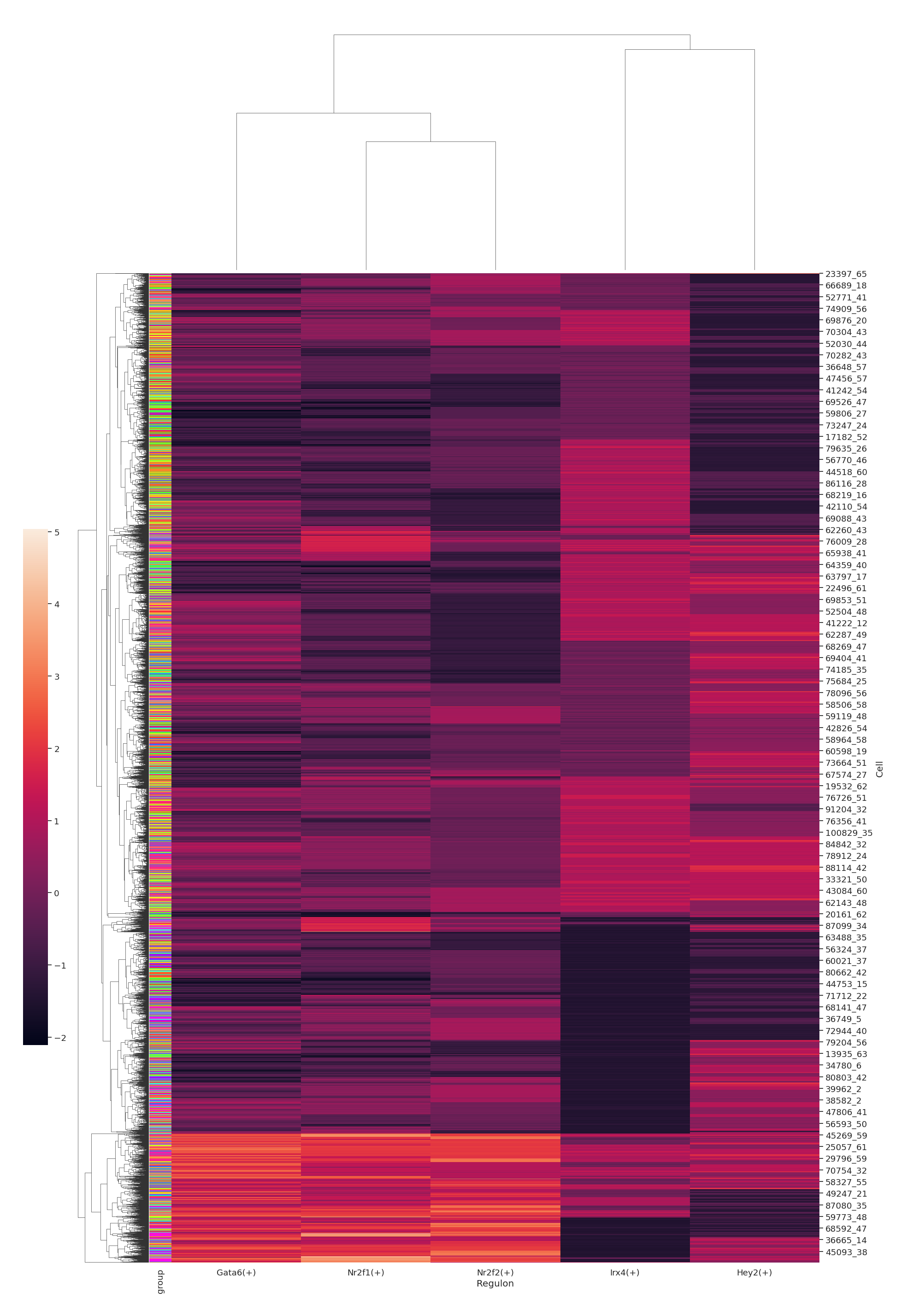
data.plt.auc_heatmap visualize the activity levels of regulons across cells, allowing for easy comparison and identification of trends or patterns. By clustering the cells based on regulon activities, one can see whether there are groups of cells that tend to have the same regulons active, and reveal the network states that are recurrent across multiple cells.
[7]:
data.plt.auc_heatmap(network_res_key='regulatory_network_inference', width=28, height=28)
[2023-11-15 18:39:42][Stereo][33882][MainThread][140148124804928][plot_collection][82][INFO]: register plot_func auc_heatmap to <stereo.plots.plot_collection.PlotCollection object at 0x7f7655587af0>
[2023-11-15 18:39:42][Stereo][33882][MainThread][140148124804928][plot_grn][263][INFO]: Generating auc heatmap plot
[7]:
<seaborn.matrix.ClusterGrid at 0x7f76778e31f0>

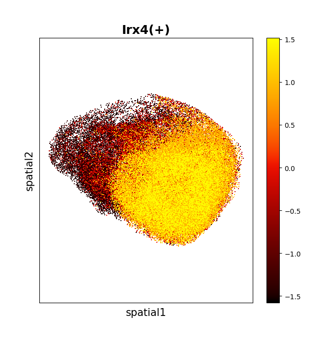
Plot the spatial distribution of the regulon activity level, with each point representing a spatial location and the color indicating the AUC value of the corresponding regulon via data.plt.spatial_scatter_by_regulon.
[8]:
data.plt.spatial_scatter_by_regulon(
reg_name='Irx4(+)',
network_res_key='regulatory_network_inference',
dot_size=2,
show_plotting_scale=False
)
[2023-11-15 18:46:08][Stereo][33882][MainThread][140148124804928][plot_collection][82][INFO]: register plot_func spatial_scatter_by_regulon to <stereo.plots.plot_collection.PlotCollection object at 0x7f7655587af0>
[2023-11-15 18:46:08][Stereo][33882][MainThread][140148124804928][plot_grn][331][INFO]: Please adjust the dot_size to prevent dots from covering each other
[8]:
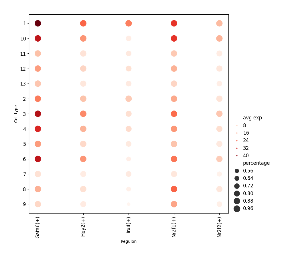
data.plt.grn_dotplot shows the expression level of regulons in different cell types. Note that the clustering of cells should be done, or the information of cell classification should be given beforehand.
[9]:
# normalization
data.tl.normalize_total(target_sum=10000)
data.tl.log1p()
data.tl.scale(max_value=10, zero_center=True)
# embedding and clustering
data.tl.pca(use_highly_genes=False, n_pcs=30, res_key='pca')
data.tl.neighbors(pca_res_key='pca', n_pcs=30, res_key='neighbors')
data.tl.leiden(neighbors_res_key='neighbors', res_key='leiden')
[2023-11-15 18:46:10][Stereo][33882][MainThread][140148124804928][st_pipeline][41][INFO]: start to run normalize_total...
[2023-11-15 18:46:11][Stereo][33882][MainThread][140148124804928][st_pipeline][44][INFO]: normalize_total end, consume time 0.2990s.
[2023-11-15 18:46:11][Stereo][33882][MainThread][140148124804928][st_pipeline][41][INFO]: start to run log1p...
[2023-11-15 18:46:12][Stereo][33882][MainThread][140148124804928][st_pipeline][44][INFO]: log1p end, consume time 1.2193s.
[2023-11-15 18:46:12][Stereo][33882][MainThread][140148124804928][st_pipeline][41][INFO]: start to run scale...
[2023-11-15 18:46:58][Stereo][33882][MainThread][140148124804928][scale][53][INFO]: Truncate at max_value 10
[2023-11-15 18:47:04][Stereo][33882][MainThread][140148124804928][st_pipeline][44][INFO]: scale end, consume time 52.1200s.
[2023-11-15 18:47:04][Stereo][33882][MainThread][140148124804928][st_pipeline][41][INFO]: start to run pca...
[2023-11-15 18:47:50][Stereo][33882][MainThread][140148124804928][st_pipeline][44][INFO]: pca end, consume time 46.5190s.
[2023-11-15 18:47:50][Stereo][33882][MainThread][140148124804928][st_pipeline][41][INFO]: start to run neighbors...
[2023-11-15 18:48:37][Stereo][33882][MainThread][140148124804928][st_pipeline][44][INFO]: neighbors end, consume time 46.7566s.
[2023-11-15 18:48:37][Stereo][33882][MainThread][140148124804928][st_pipeline][41][INFO]: start to run leiden...
[2023-11-15 18:49:09][Stereo][33882][MainThread][140148124804928][st_pipeline][44][INFO]: leiden end, consume time 32.1148s.
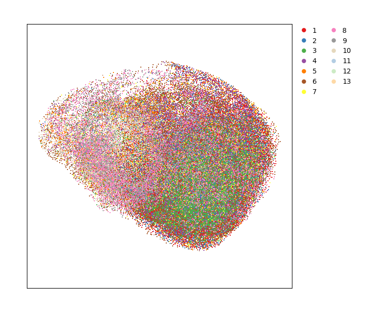
[10]:
# scatter plot
data.plt.cluster_scatter(res_key='leiden', dot_size=2, show_plotting_scale=False)
[10]:
[11]:
data.plt.grn_dotplot(cluster_res_key='leiden', network_res_key='regulatory_network_inference')
[2023-11-15 18:49:10][Stereo][33882][MainThread][140148124804928][plot_collection][82][INFO]: register plot_func grn_dotplot to <stereo.plots.plot_collection.PlotCollection object at 0x7f7655587af0>
INFO:matplotlib.category:Using categorical units to plot a list of strings that are all parsable as floats or dates. If these strings should be plotted as numbers, cast to the appropriate data type before plotting.
INFO:matplotlib.category:Using categorical units to plot a list of strings that are all parsable as floats or dates. If these strings should be plotted as numbers, cast to the appropriate data type before plotting.
[11]:
data.plt.auc_heatmap_by_group function will first identify regulons with the highest activity of each cell type (by setting top_n_feature value), then perform z-score calculation to visualize the AUC scores as heatmap.
[13]:
data.plt.auc_heatmap_by_group(
network_res_key='regulatory_network_inference',
cluster_res_key='leiden',
top_n_feature=5
)
[13]:
<seaborn.matrix.ClusterGrid at 0x7f76b8408c70>