Quick Start (Cell Bin)
In this case, we use the .cellbin.gef file of mouse brain generated by Stereo-seq for downstream analysis.
More information of GEF file is in the documentation. Usually, we recommend using GEF whose speed of being read is much faster than GEM.
Reading data
Firstly, download our example data and import Stereopy.
[1]:
import stereo as st
import warnings
warnings.filterwarnings('ignore')
Get the version information of Stereopy.
[2]:
st.__version__
[2]:
'1.3.1'
Get attributes of the GEF file
[3]:
data_path = '../../data/SS200000135TL_D1.cellbin.gef'
st.io.read_gef_info(data_path)
[2024-07-30 10:03:28][Stereo][215369][MainThread][139961767442240][reader][1412][INFO]: This is GEF file which contains cell bin infomation.
[2024-07-30 10:03:28][Stereo][215369][MainThread][139961767442240][reader][1413][INFO]: bin_type: cell_bins
[2024-07-30 10:03:28][Stereo][215369][MainThread][139961767442240][reader][1419][INFO]: Number of cells: 57133
[2024-07-30 10:03:28][Stereo][215369][MainThread][139961767442240][reader][1422][INFO]: Number of gene: 24670
[2024-07-30 10:03:28][Stereo][215369][MainThread][139961767442240][reader][1425][INFO]: Resolution: 500
[2024-07-30 10:03:28][Stereo][215369][MainThread][139961767442240][reader][1428][INFO]: offsetX: 0
[2024-07-30 10:03:28][Stereo][215369][MainThread][139961767442240][reader][1431][INFO]: offsetY: 0
[2024-07-30 10:03:28][Stereo][215369][MainThread][139961767442240][reader][1434][INFO]: Average number of genes: 223.460693359375
[2024-07-30 10:03:28][Stereo][215369][MainThread][139961767442240][reader][1437][INFO]: Maximum number of genes: 1046
[2024-07-30 10:03:28][Stereo][215369][MainThread][139961767442240][reader][1440][INFO]: Average expression: 399.17034912109375
[2024-07-30 10:03:28][Stereo][215369][MainThread][139961767442240][reader][1443][INFO]: Maximum expression: 2337
version is 0.7.14
[3]:
{'cell_num': 57133,
'gene_num': 24670,
'resolution': 500,
'offsetX': 0,
'offsetY': 0,
'averageGeneCount': 223.4607,
'maxGeneCount': 1046,
'averageExpCount': 399.17035,
'maxExpCount': 2337}
Note
bin_type should be set to 'cell_bins', if read a GEF file of .cellbin.gef, which is significantly different from Square Bin.
Load data to generate a StereoExpData object.
[4]:
data = st.io.read_gef(file_path=data_path, bin_type='cell_bins')
# simply type the varibale to get related information
data
[2024-07-30 10:03:28][Stereo][215369][MainThread][139961767442240][reader][1170][INFO]: read_gef begin ...
version is 0.7.14
[2024-07-30 10:03:29][Stereo][215369][MainThread][139961767442240][reader][1412][INFO]: This is GEF file which contains cell bin infomation.
[2024-07-30 10:03:29][Stereo][215369][MainThread][139961767442240][reader][1413][INFO]: bin_type: cell_bins
[2024-07-30 10:03:29][Stereo][215369][MainThread][139961767442240][reader][1419][INFO]: Number of cells: 57133
[2024-07-30 10:03:29][Stereo][215369][MainThread][139961767442240][reader][1422][INFO]: Number of gene: 24670
[2024-07-30 10:03:29][Stereo][215369][MainThread][139961767442240][reader][1425][INFO]: Resolution: 500
[2024-07-30 10:03:29][Stereo][215369][MainThread][139961767442240][reader][1428][INFO]: offsetX: 0
[2024-07-30 10:03:29][Stereo][215369][MainThread][139961767442240][reader][1431][INFO]: offsetY: 0
[2024-07-30 10:03:29][Stereo][215369][MainThread][139961767442240][reader][1434][INFO]: Average number of genes: 223.460693359375
[2024-07-30 10:03:29][Stereo][215369][MainThread][139961767442240][reader][1437][INFO]: Maximum number of genes: 1046
[2024-07-30 10:03:29][Stereo][215369][MainThread][139961767442240][reader][1440][INFO]: Average expression: 399.17034912109375
[2024-07-30 10:03:29][Stereo][215369][MainThread][139961767442240][reader][1443][INFO]: Maximum expression: 2337
[2024-07-30 10:03:29][Stereo][215369][MainThread][139961767442240][reader][1259][INFO]: the matrix has 57133 cells, and 24670 genes.
version is 0.7.14
[4]:
StereoExpData object with n_cells X n_genes = 57133 X 24670
bin_type: cell_bins
offset_x = None
offset_y = None
cells: ['cell_name', 'dnbCount', 'area']
genes: ['gene_name']
result: []
Preprocessing
Data preprocessing includes three modules: quality control, filtering and normalization.
Quality Control
This module calculates the quality distribution of original data, using three indicators:
total_counts - the total counts per cell;
n_genes_by_counts - the number of genes expressed in count maxtrix;
pct_countss_mt - the percentage of counts in mitochondrial genes.
[5]:
data.tl.cal_qc()
[2024-07-30 10:03:29][Stereo][215369][MainThread][139961767442240][st_pipeline][41][INFO]: start to run cal_qc...
[2024-07-30 10:03:29][Stereo][215369][MainThread][139961767442240][st_pipeline][44][INFO]: cal_qc end, consume time 0.1702s.
Show the violin figure of QC distribution.
[6]:
data.plt.violin()
[6]:

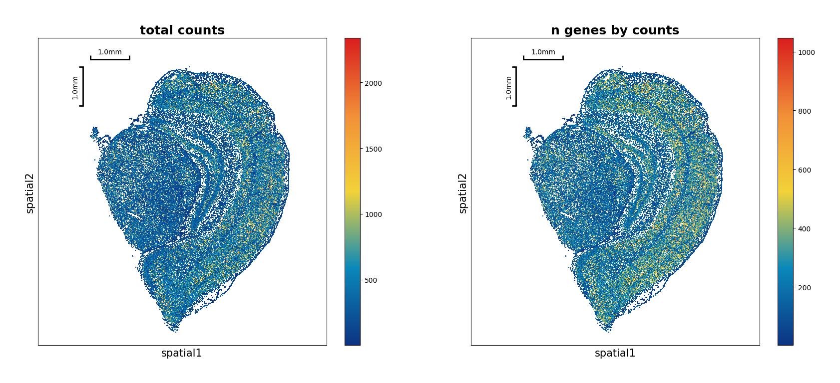
Show the spatial scatter figure of QC distribution.
[7]:
data.plt.spatial_scatter()
[7]:
Filtering
Three basic methods are provided to filter data maxtrix:
data.tl.filter_cells, data.tl.filter_genes, data.tl.filter_coordinates.
We filter cells based on quality control indicators which have been calculated in QC part. Beforehand, observe the distribution of cells according to scatter plots.
[8]:
data.plt.genes_count()
[8]:

Remove cells that have too many mitochondrial genes expressed, without enough genes expressed, and out of count range.
[9]:
data.tl.filter_cells(
min_counts=200,
min_genes=3,
max_genes=2500,
pct_counts_mt=5,
inplace=True
)
data
[2024-07-30 10:03:33][Stereo][215369][MainThread][139961767442240][st_pipeline][41][INFO]: start to run filter_cells...
[2024-07-30 10:03:33][Stereo][215369][MainThread][139961767442240][st_pipeline][44][INFO]: filter_cells end, consume time 0.1045s.
[9]:
StereoExpData object with n_cells X n_genes = 41948 X 24670
bin_type: cell_bins
offset_x = None
offset_y = None
cells: ['cell_name', 'dnbCount', 'area', 'total_counts', 'n_genes_by_counts', 'pct_counts_mt']
genes: ['gene_name', 'n_cells', 'n_counts', 'mean_umi']
result: []
Note
We strongly suggest to use self.raw to record the raw gene expression matrix which has been gone through basic processing, as an essential data set for subsequent differential testing and multiple analysis.
So in order to save the data and recall it conveniently, you can save the raw expression matrix by data.tl.raw_checkpoint().
[10]:
data.tl.raw_checkpoint()
[11]:
data.tl.raw
[11]:
StereoExpData object with n_cells X n_genes = 41948 X 24670
bin_type: cell_bins
offset_x = None
offset_y = None
cells: ['cell_name', 'dnbCount', 'area', 'total_counts', 'n_genes_by_counts', 'pct_counts_mt']
genes: ['gene_name', 'n_cells', 'n_counts', 'mean_umi']
result: []
Note
When you want to get raw data, just run data.tl.reset_raw_data().
Normalization
In this module, you can choose from following common methods of standardization:
Note
If the parameter inplace is set to True by default, expression matrix data will be replaced by the corresponding result(here replaced by the normalized result), otherwise unchanged.
Run a combination method of normalize_total and log1p to normalize gene expression matrix as below:
[12]:
# inplace is set to True by default
data.tl.normalize_total()
data.tl.log1p()
[2024-07-30 10:03:33][Stereo][215369][MainThread][139961767442240][st_pipeline][41][INFO]: start to run normalize_total...
[2024-07-30 10:03:33][Stereo][215369][MainThread][139961767442240][st_pipeline][44][INFO]: normalize_total end, consume time 0.0537s.
[2024-07-30 10:03:33][Stereo][215369][MainThread][139961767442240][st_pipeline][41][INFO]: start to run log1p...
[2024-07-30 10:03:33][Stereo][215369][MainThread][139961767442240][st_pipeline][44][INFO]: log1p end, consume time 0.0801s.
If you use data.tl.sctransform which includes the function of finding highly variable genes, you do not need to run data.tl.highly_variable_genes. In the subsequent data.tl.pca method, the parameter use_highly_genes has to be set as False. In brief, whether to use highly variable genes to run PCA depends on filter_hvgs in the normalization of scTransform. Learn more about
scTransform.
Highly variable genes
Identify highly variable genes in cells.
[13]:
data.tl.highly_variable_genes(
min_mean=0.0125,
max_mean=3,
min_disp=0.5,
n_top_genes=2000,
res_key='highly_variable_genes'
)
[2024-07-30 10:03:33][Stereo][215369][MainThread][139961767442240][st_pipeline][41][INFO]: start to run highly_variable_genes...
[2024-07-30 10:03:33][Stereo][215369][MainThread][139961767442240][st_pipeline][44][INFO]: highly_variable_genes end, consume time 0.4253s.
If data.tl.scale(zero_center=False) is used, sparse matrix will be used for calculation, which can greatly reduce the memory required for running.
[14]:
# remember to choose a res_key when plot
data.plt.highly_variable_genes(res_key='highly_variable_genes')
[14]:

Scale each gene to unit variance. Clip values exceeding standard deviation 10. If data.tl.scale(zero_center=False) is used, sparse matrix will be used for calculation, which can greatly reduce the memory required for running.
[15]:
data.tl.scale()
[2024-07-30 10:03:34][Stereo][215369][MainThread][139961767442240][st_pipeline][41][INFO]: start to run scale...
[2024-07-30 10:03:34][Stereo][215369][MainThread][139961767442240][st_pipeline][44][INFO]: scale end, consume time 0.1046s.
Embedding
PCA (Principal component analysis)
As a statistical technique for reducing dimensionality of a data set, PCA finds the max axes of greatest variation, which preserve as much information as possible. Notice that if set parameter use_highly_genes to True, only highly variable genes are used to run.
[16]:
data.tl.pca(
use_highly_genes=True,
n_pcs=30,
res_key='pca'
)
[2024-07-30 10:03:34][Stereo][215369][MainThread][139961767442240][st_pipeline][41][INFO]: start to run pca...
[2024-07-30 10:03:34][Stereo][215369][MainThread][139961767442240][dim_reduce][78][WARNING]: svd_solver: auto can not be used with sparse input.
Use "arpack" (the default) instead.
[2024-07-30 10:03:35][Stereo][215369][MainThread][139961767442240][st_pipeline][44][INFO]: pca end, consume time 0.9816s.
When the parameter res_key arises, the corresponding result will be stored automatically, simply check:
data.tl.key_record
We can plot the elbow to help us to determine how to choose PCs to be used.
[17]:
data.plt.elbow(pca_res_key='pca')
[2024-07-30 10:03:35][Stereo][215369][MainThread][139961767442240][plot_collection][84][INFO]: register plot_func elbow to <stereo.plots.plot_collection.PlotCollection object at 0x7f4ae8da12e0>
[17]:

Neighborhood graph
After PCA, we compute the neighborhood graph of cells using the PCA representation of the expression matrix.
[18]:
data.tl.neighbors(pca_res_key='pca', res_key='neighbors')
[2024-07-30 10:03:36][Stereo][215369][MainThread][139961767442240][st_pipeline][41][INFO]: start to run neighbors...
2024-07-30 10:03:38.607999: W tensorflow/stream_executor/platform/default/dso_loader.cc:64] Could not load dynamic library 'libcudart.so.11.0'; dlerror: libcudart.so.11.0: cannot open shared object file: No such file or directory; LD_LIBRARY_PATH: /root/miniforge3/envs/stereopy/lib/python3.8/site-packages/cv2/../../lib64:
2024-07-30 10:03:38.608033: I tensorflow/stream_executor/cuda/cudart_stub.cc:29] Ignore above cudart dlerror if you do not have a GPU set up on your machine.
[2024-07-30 10:03:50][Stereo][215369][MainThread][139961767442240][st_pipeline][44][INFO]: neighbors end, consume time 14.5194s.
In addition, we also provide data.tl.spatial_neighbors function to compute a spatial neighbors graph.
UMAP
It’s strongly to suggest embedding the graph in two dimensions using UMAP.
[19]:
data.tl.umap(
pca_res_key='pca',
neighbors_res_key='neighbors',
res_key='umap'
)
[2024-07-30 10:03:50][Stereo][215369][MainThread][139961767442240][st_pipeline][41][INFO]: start to run umap...
completed 0 / 200 epochs
completed 20 / 200 epochs
completed 40 / 200 epochs
completed 60 / 200 epochs
completed 80 / 200 epochs
completed 100 / 200 epochs
completed 120 / 200 epochs
completed 140 / 200 epochs
completed 160 / 200 epochs
completed 180 / 200 epochs
[2024-07-30 10:04:03][Stereo][215369][MainThread][139961767442240][st_pipeline][44][INFO]: umap end, consume time 13.2834s.
[20]:
# plot the umap result of two genes: 'Atpif1' and 'Tmsb4x'
data.plt.umap(gene_names=['Atpif1', 'Tmsb4x'], res_key='umap')
[20]:

Clustering
Currently we provide three common clustering methods, including Leiden, Louvain and Phenograph.
In this tool, you can re-run the normalization method before clustering if the parameter normalize_method is not None. Then by default, we perform PCA to reduce the dimensionalites of the new normalization result, and use top 30 pcs to run clustering.
At this stage, we strongly recommend using leiden.
Leiden
Simply run:
[21]:
data.tl.leiden(neighbors_res_key='neighbors',res_key='leiden')
[2024-07-30 10:04:05][Stereo][215369][MainThread][139961767442240][st_pipeline][41][INFO]: start to run leiden...
[2024-07-30 10:04:26][Stereo][215369][MainThread][139961767442240][st_pipeline][44][INFO]: leiden end, consume time 21.0193s.
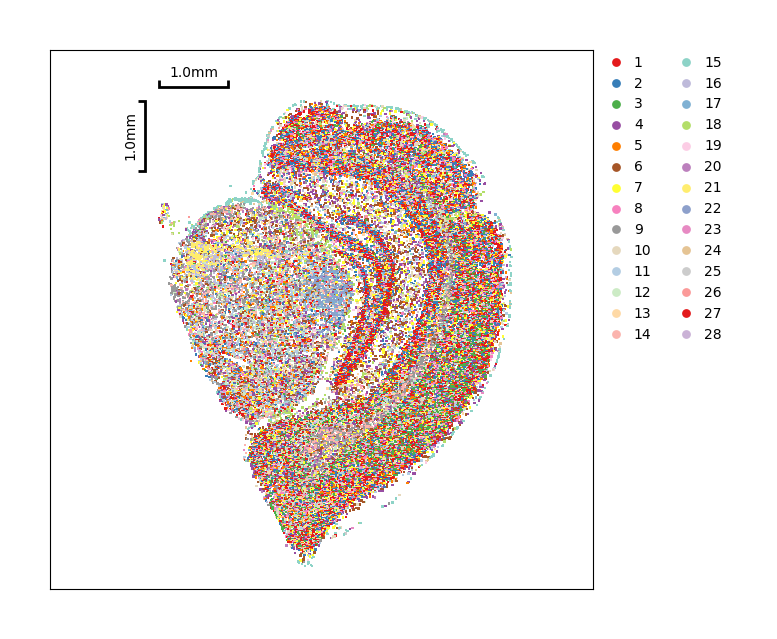
Show the spatial distribution of the clustering result.
[22]:
data.plt.cluster_scatter(res_key='leiden')
[22]:

You also can only show partial clustering result.
[23]:
data.plt.cluster_scatter(res_key='leiden', groups=['1', '2'])
[23]:

We can visulize the detail of cells base on clustering result. If set the parameter base_image, it will draw the ssDNA image as background and you can set transparency of foreground by the parameter fg_alpha.
we can also export this plot as SVG or PDF, more detail in API.
[24]:
data.plt.cells_plotting(color_by='cluster', color_key='leiden')
#data.plt.cells_plotting(color_by='cluster', color_key='leiden', base_image='./data/SS200000135TL_D1_regist.tif', fg_alpha=0.8)
[24]:
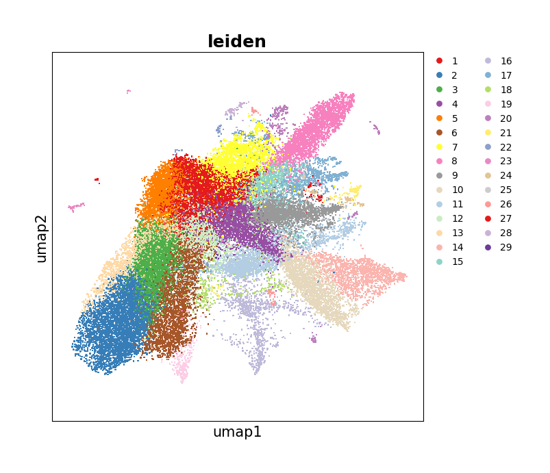
Show the UMAP spatial distribution of the clustering result.
[25]:
data.plt.umap(res_key='umap', cluster_key='leiden')
[25]:
data.plt.interact_cluster generates an interact module from Jupyter Notebook and basic interactive manipulations could be done here. Simple clicks help you finish a series of operations, inclusing moving, tailoring, dyeing, saving and etc., over different clustering groups. More about in Interactive cluster.
[26]:
data.plt.interact_cluster(res_key='leiden')
[26]:
Louvain
When clustering by Louvain algorithm, just run:
[27]:
data.tl.louvain(neighbors_res_key='neighbors', res_key='louvain')
[2024-07-30 10:05:00][Stereo][215369][MainThread][139961767442240][st_pipeline][41][INFO]: start to run louvain...
[2024-07-30 10:05:00][Stereo][215369][MainThread][139961767442240][_louvain][109][INFO]: using the "louvain" package of Traag (2017)
[2024-07-30 10:05:05][Stereo][215369][MainThread][139961767442240][st_pipeline][44][INFO]: louvain end, consume time 4.8652s.
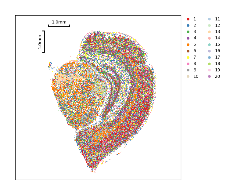
Show the spatial distribution of Louvain clustering.
[28]:
data.plt.cluster_scatter(res_key='louvain')
[28]:
Same as Leiden, you can show detail of cells by the data.plt.cells_plotting.
Phenograph
When clustering by Phenograph algorithm, just run:
[29]:
data.tl.phenograph(phenograph_k=30, pca_res_key='pca', res_key='phenograph')
[2024-07-30 10:05:06][Stereo][215369][MainThread][139961767442240][st_pipeline][41][INFO]: start to run phenograph...
Finding 30 nearest neighbors using minkowski metric and 'auto' algorithm
Neighbors computed in 2.9804258346557617 seconds
Jaccard graph constructed in 2.906126022338867 seconds
Running Leiden optimization
Leiden completed in 22.498373985290527 seconds
Sorting communities by size, please wait ...
PhenoGraph completed in 29.742438316345215 seconds
[2024-07-30 10:05:35][Stereo][215369][MainThread][139961767442240][st_pipeline][44][INFO]: phenograph end, consume time 29.9126s.
Show the spatial distribution of Phenograph clustering.
[30]:
data.plt.cluster_scatter(res_key='phenograph')
[30]:
Same as Leiden, you can show detail of cells by data.plt.cells_plotting.
Find Marker Genes
Hypothesis test is used to compute a ranking of differential genes among clusters. The raw count of express matrix which has been saved in self.raw by data.tl.raw_checkpoint() and highly variable genes are two optional data sets used to find marker genes.
Here supports two methods, t_test and wilcoxon_test, to find marker genes between pairs among all clusters. T-test as a more common and simple approach to do so.
[31]:
data.tl.find_marker_genes(
cluster_res_key='phenograph',
method='t_test',
use_highly_genes=False,
use_raw=True
)
[2024-07-30 10:05:36][Stereo][215369][MainThread][139961767442240][st_pipeline][41][INFO]: start to run find_marker_genes...
[2024-07-30 10:05:37][Stereo][215369][MainThread][139961767442240][tool_base][122][INFO]: read group information, grouping by group column.
[2024-07-30 10:05:37][Stereo][215369][MainThread][139961767442240][tool_base][151][INFO]: start to run...
[2024-07-30 10:05:39][Stereo][215369][MainThread][139961767442240][tool_base][153][INFO]: end to run.
[2024-07-30 10:05:39][Stereo][215369][MainThread][139961767442240][st_pipeline][44][INFO]: find_marker_genes end, consume time 3.0699s.
Display the ranking and scores of top 10 marker genes in each group.
[32]:
data.plt.marker_genes_text(
res_key='marker_genes',
markers_num=10,
sort_key='scores'
)
[32]:
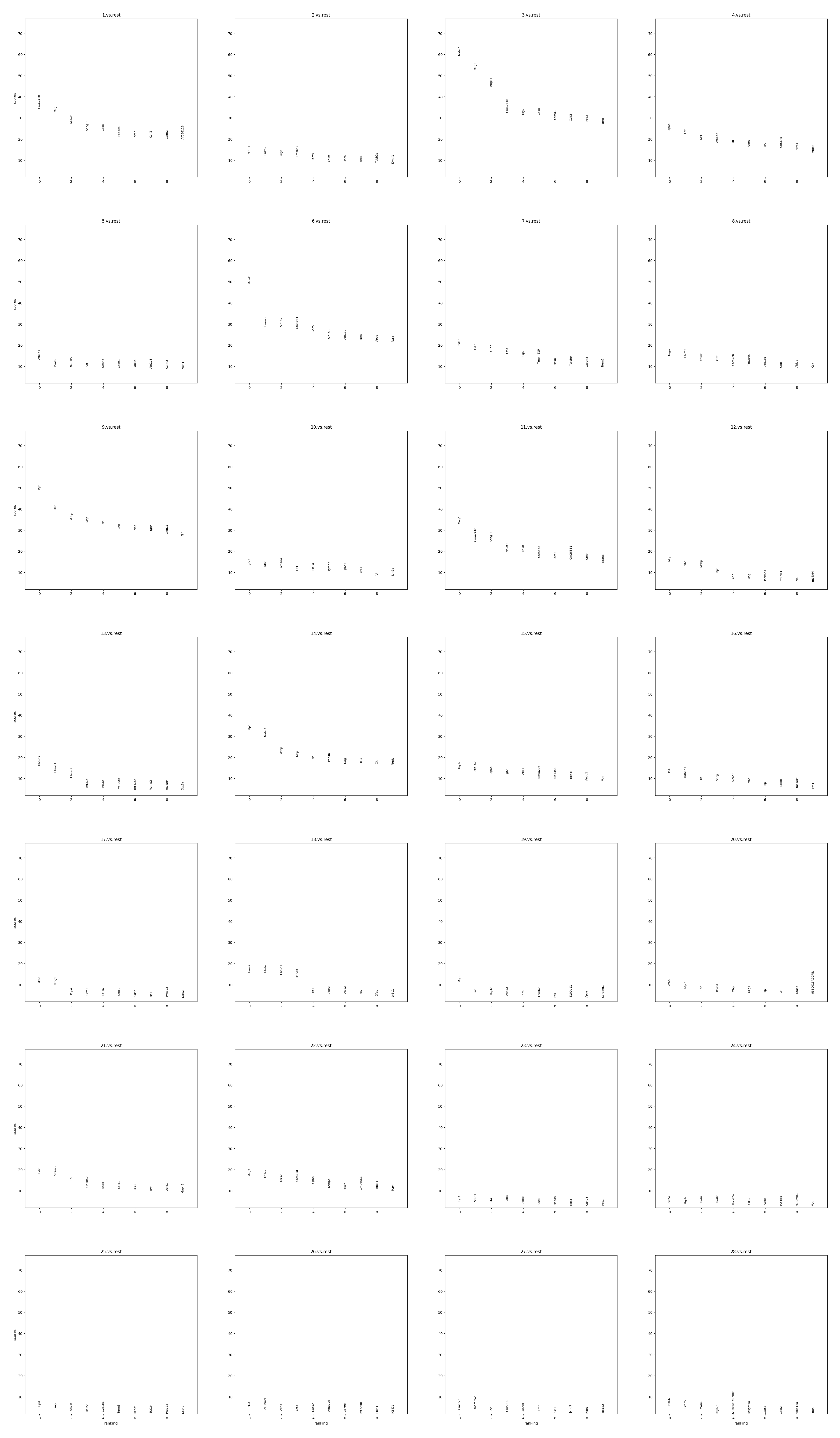
Display the scatter plot of top 5 marker genes in each group.
[33]:
data.plt.marker_genes_scatter(res_key='marker_genes', markers_num=5)
[33]:

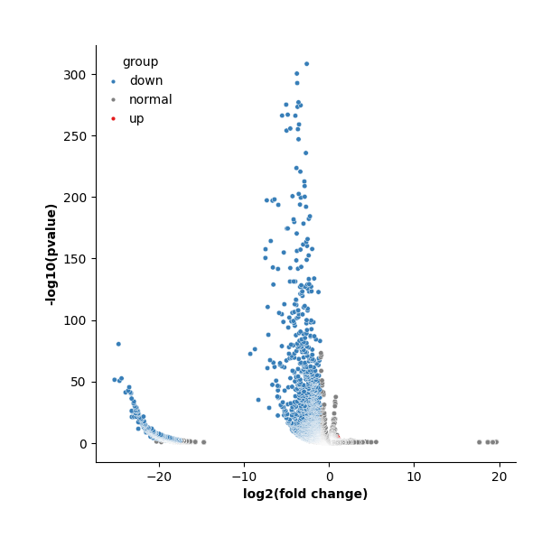
Meanwhile, display the volcano plot of a specific group versus to the rest.
[34]:
data.plt.marker_gene_volcano(group_name='2.vs.rest', vlines=False)
[34]:
You can also filter out genes based on log fold change and fraction of genes expressing the gene within and outside each group.
[35]:
data.tl.filter_marker_genes(
marker_genes_res_key='marker_genes',
min_fold_change=1,
min_in_group_fraction=0.25,
max_out_group_fraction=0.5,
res_key='marker_genes_filtered'
)
[2024-07-30 10:05:45][Stereo][215369][MainThread][139961767442240][st_pipeline][41][INFO]: start to run filter_marker_genes...
[2024-07-30 10:05:46][Stereo][215369][MainThread][139961767442240][st_pipeline][44][INFO]: filter_marker_genes end, consume time 1.0790s.
Annotation
After finding marker genes, we can annotate clustering results by using data.tl.annotation or data.plt.interact_annotation_cluster.
[36]:
data.plt.interact_annotation_cluster(
res_cluster_key='leiden',
res_marker_gene_key='marker_genes',
res_key='leiden_annotation'
)
[36]:
Use command lines to annotate clusters:
[37]:
annotation_dict = {
'1':'a',
'2':'b',
'3':'c',
'4':'d',
'5':'e',
'6':'f',
'7':'g',
'8':'h',
'9':'i',
'10':'j',
'11':'k',
'12':'l',
'13':'m',
'14':'n',
'15':'o',
'16':'p',
'17':'q',
'18':'r',
'19':'s',
'20':'t',
'21':'u',
'22':'v',
'23':'w',
'24':'x',
'25':'y'
}
data.tl.annotation(
annotation_information=annotation_dict,
cluster_res_key='leiden',
res_key='anno_leiden'
)
[2024-07-30 10:05:48][Stereo][215369][MainThread][139961767442240][st_pipeline][41][INFO]: start to run annotation...
[2024-07-30 10:05:48][Stereo][215369][MainThread][139961767442240][st_pipeline][44][INFO]: annotation end, consume time 0.2441s.
[38]:
data.plt.cluster_scatter(res_key='anno_leiden')
[38]:
