Apply spaTrack to infer cell transitions across multiple time points in spatial transcriptomic data from the mouse midbrain

Multiple ST tissue sections obtained at different timepoints offer a valuable opportunity to gain a deeper understanding of cell transitions during organ development, such as mouse midbrain development and zebrafish embryogenesis. spaTrack can provide a novel strategy to infer cell tracing across multiple tissue sections based on an unbalanced and structured optimal transport algorithm by direct mapping cells among samples without integrating data. This approach is designed for cases where multiple sections containing the same cell types.In this tutorial, We use mouse midbrain ST data to demonstrate cell transfer across ST slides of multiple time points.The data can be downloaded from our example data.

import warnings
warnings.filterwarnings("ignore")

import stereo as st
from stereo.core.ms_data import MSData
from stereo.core.ms_pipeline import slice_generator

Load data

In this data, the cell type information is stored in data.cells['annotation'] or data.adata.obs['annotation'] and the spatial coordinates is stored by key ‘spatial’.

data_path = '../../data/04.mouse.midbrain.three.time/04.mouse.midbrain.three.time.point.ST.exp.h5ad'

data = st.io.read_h5ad(data_path, spatial_key='spatial')
data

AnnData object with n_obs × n_vars = 4528 × 24045
    obs: 'annotation', 'Time point', 'x', 'y', 'batch', 'cell_id'
    uns: 'sn'
    obsm: 'spatial'

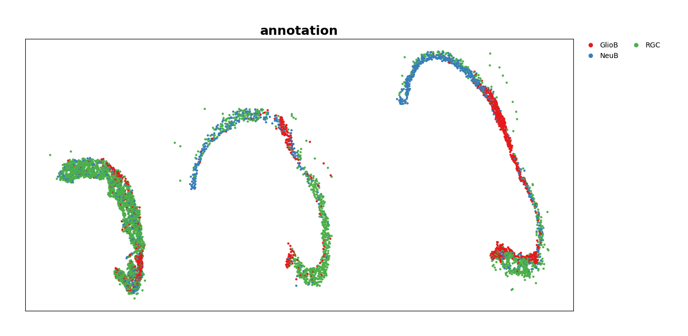
Visualzation of mouse midbrain ST data of three time points.

data.plt.cluster_scatter(res_key='annotation', width=1400, height=700, marker='o', dot_size=10, show_plotting_scale=False, invert_y=False)

Calculate transition probability across sections

Create a multi-sample data structure

Create a multi-sample data structure along the time points specified by obs-key Time point, in this case, the data will be split into 3 single samples with 3 different Time point.

ms_data = MSData.to_msdata(data, batch_key='Time point')
ms_data

ms_data: {'E12.5': (2237, 24045), 'E14.5': (953, 24045), 'E16.5': (1338, 24045)}
num_slice: 3
names: ['E12.5', 'E14.5', 'E16.5']
merged_data: None
obs: []
var: []
relationship: other
var_type: intersect to 0
current_mode: integrate
current_scope: scope_[0,1,2]
scopes_data: []
mss: []

Get An object of spaTrack

spt = ms_data.tl.ms_spa_track(cluster_res_key='annotation')

2024-11-07 10:05:26.178946: W tensorflow/compiler/tf2tensorrt/utils/py_utils.cc:38] TF-TRT Warning: Could not find TensorRT

Calculate transition probability

spaTrack infers cell tracing across multiple ST sections based on an unbalanced and structured optimal transport algorithm. We can calculate the transfer matrix between two ST sections using the spt.transfer_matrix function. Additionally, the transition probability between two sections can be calculated using spt.map_data. To obtain complete results across multiple sections, spt.generate_animate_input is used to integrate the transition probability results.

spt.transfer_matrix(data1_index='E12.5', data2_index='E14.5', epsilon=0.01, alpha=0.5)
spt.transfer_matrix(data1_index='E14.5', data2_index='E16.5', epsilon=0.01, alpha=0.5)

We also can obtain the result containing cell transition probability among three ST sections.

spt.generate_animate_input(data_indices=['E12.5', 'E14.5', 'E16.5'], time_key='Time point')

ms_data.tl.result['spa_track']['transfer_data'].head()

	slice1	slice2	slice3	slice1_annotation	slice2_annotation	slice3_annotation	slice1_x	slice2_x	slice3_x	slice1_y	slice2_y	slice3_y	k_line_12	b_line_12	k_line_23	b_line_23	pi_value1	pi_value2
0	CELL.100034_1	CELL.174282_3	CELL.6090_2	RGC	GlioB	RGC	2829.0	7709.0	14163.004072	-10000.0	-9508.0	-9438.505655	0.100820	-10285.218852	0.010768	-9591.007680	0.000043	0.000118
1	CELL.105423_1	CELL.174282_3	CELL.6090_2	NeuB	GlioB	RGC	2325.0	7709.0	14163.004072	-9678.5	-9508.0	-9438.505655	0.031668	-9752.127879	0.010768	-9591.007680	0.000076	0.000118
2	CELL.100795_1	CELL.174235_3	CELL.5906_2	RGC	RGC	GlioB	2893.0	8825.0	15324.653342	-9946.5	-9519.0	-9458.827390	0.072067	-10154.989127	0.009258	-9600.700247	0.000055	0.000075
3	CELL.105209_1	CELL.174235_3	CELL.5906_2	GlioB	RGC	GlioB	3007.0	8825.0	15324.653342	-9693.0	-9519.0	-9458.827390	0.029907	-9782.930904	0.009258	-9600.700247	0.000046	0.000075
4	CELL.114403_1	CELL.174235_3	CELL.5906_2	RGC	RGC	GlioB	2856.0	8825.0	15324.653342	-8887.5	-9519.0	-9458.827390	-0.105797	-8585.344865	0.009258	-9600.700247	0.000065	0.000075

The transfer_data above contains comprehensive results from multiple sections. In the dataframe, First three columns represent the CellID in slice1, slice2, and slice3 with the maximum transition probability among them. The pi_value1 represents the maximum transition probability value between the CellID in slice1 and slice2. Similarly, the pi_value2 represents the maximum transition probability value between the CellID in slice2 and slice3. The k_line and b_line represent slopes and intercepts of lines connecting two cells used by spt.animate_transfer() function to display dynamic figure. Users have the option to filter the maximum transition probability values based on their distribution.

Visualze cell transfer by dynamic figure

A necessary dependency needs to be installed:

pip install nbformat

spt.plot.animate_transfer(
    data_indices=['E12.5', 'E14.5', 'E16.5'],
    time_key ='Time point',
    save_path='./cell.transfer.animation.html',
)

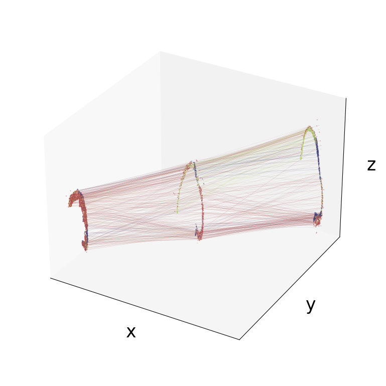
Visualize cell transfer by 3D figure

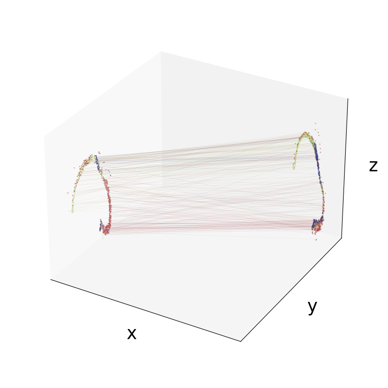
We can visualize the three sections and the line cells with the maximum transition probability in a 3D space.

spt.plot.visual_3D_mapping_3(
    data_indices=['E12.5', 'E14.5', 'E16.5'],
    dot_size=0.8,
    line_width=0.06
)

We can visualize specific two consecutive sections after calculating the transition probability across the sections. Now,we can obtain the file containing cell transition probability between section 1(E14.5) and section 2(E16.5).

spt.map_data(data1_index='E14.5', data2_index='E16.5')

	slice1	slice2	pi_value
CELL.171967_3	CELL.171967_3	CELL.6438_2	0.000142
CELL.172008_3	CELL.172008_3	CELL.5694_2	0.000125
CELL.172028_3	CELL.172028_3	CELL.6242_2	0.000059
CELL.172036_3	CELL.172036_3	CELL.5934_2	0.000101
CELL.172085_3	CELL.172085_3	CELL.5836_2	0.000115
...	...	...	...
CELL.180529_3	CELL.180529_3	CELL.1796_2	0.000086
CELL.180537_3	CELL.180537_3	CELL.3207_2	0.000107
CELL.180539_3	CELL.180539_3	CELL.3044_2	0.000118
CELL.180540_3	CELL.180540_3	CELL.3688_2	0.000079
CELL.180550_3	CELL.180550_3	CELL.3517_2	0.000216

953 rows × 3 columns

spt.plot.visual_3D_mapping_2(
    data1_index='E14.5',
    data2_index='E16.5',
    dot_size=1,
    line_width=0.05
)

Construct gene regulation network

Here, we use data from E12.5 and E14.5 as an example to construct regulatory network between TF genes and target genes inferred along the developmental trajectory between two time points.TF genes list of Mouse and Human can be download from the link.

Torch is the necessary dependency for this function and needs to be installed first.

CPU: pip install torch==2.4.1+cpu --extra-index-url https://download.pytorch.org/whl

GPU(CUDA11): pip install torch==2.4.1+cu118 --extra-index-url https://download.pytorch.org/whl/

GPU(CUDA12): pip install torch==2.4.1+cu124 --extra-index-url https://download.pytorch.org/whl/

gr = spt.gr_training(
    data1_index='E12.5',
    data2_index='E14.5',
    tfs_path='../spaTrack/spaTrack/example.data/ms.TF.tsv',
    min_cells_1=50,         #recommend maintaining gene expression in ～ 3% of cells.
    min_cells_2=20,
    cell_generate_per_time=10000,
    cell_select_per_time=50,
    training_times=10,
    iter_times=30,
    use_gpu=False # set to True to use GPU
)

Train 10: 100%|██████████| 300/300 [03:33<00:00,  1.41it/s, train_loss=0.0144, test_loss=0.0158]
[2024-11-07 10:10:25][Stereo][1068][MainThread][140492234536768][gene_regulation][292][INFO]: Weight relationships of tfs and genes are stored in weights.csv.

Show the relationship between TF and target genes by scatter diagram.

gr.plot_scatter()

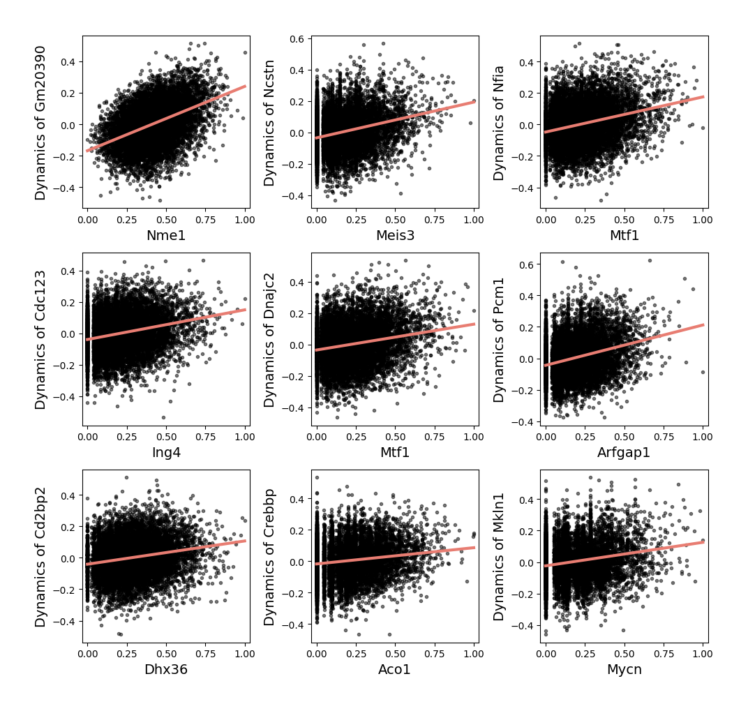
Get weights between TFs and genes.

gr.network_df

	TF	gene	weight
347	Nme1	Gm20390	0.031272
950	Meis3	Ncstn	0.021513
1197	Mtf1	Nfia	0.021020
2294	Ing4	Cdc123	0.020342
1785	Mtf1	Dnajc2	0.020236
...	...	...	...
1630	Chd1	Foxk2	0.010869
435	Creb1	Cnot8	0.010869
2862	Chd1	Kdm2a	0.010868
694	Srebf1	Vps4b	0.010868
284	Apex1	Ostc	0.010867

3000 rows × 3 columns

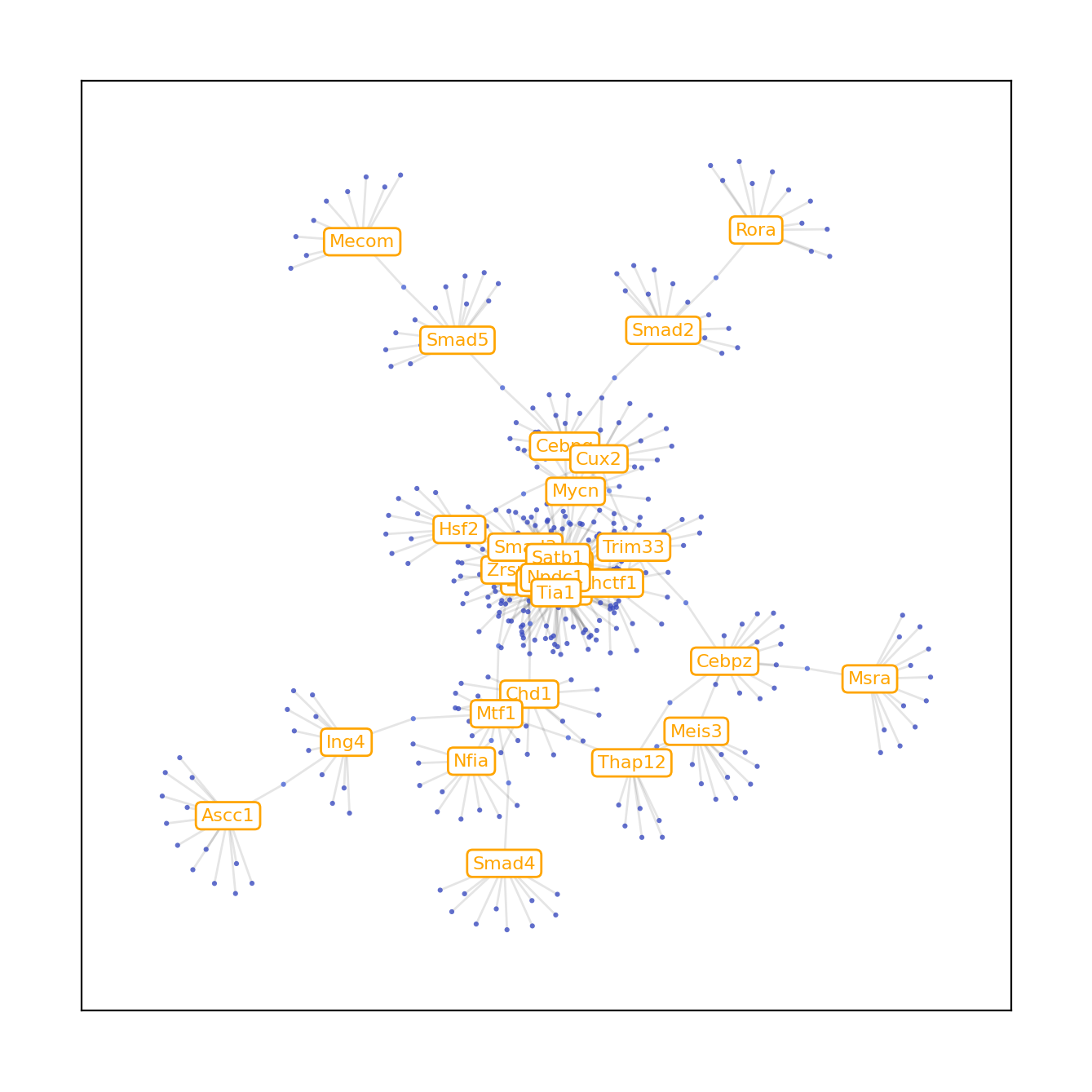
Plot the gene regulatory network diagram according to the gr.network_df.

gr.plot_gene_regulation(min_weight=0.012, min_node_num=10)

num of weight pairs after weight filtering: 1388
num of weight pairs after node_count filtering: 394